It’s widely known that implementing and optimizing GEMM (GEneral Matrix Multiplication) is fundamental when it comes to learning GPU programming. In this post, we’ll walk through the process of implementing and optimizing single-precision and mixed-precision GEMM: from a brief overview of what the operation does to advanced optimizations using Tensor Cores.

I primarily use Simon’s GEMM posts as the foundation for this work. I begin by reimplementing the kernels from Simon’s post, documenting the insights along the way, and then extend them with more recent optimization techniques. As for Tensor Core-based optimizations, I draw heavily from the notes and explanations in Alex’s post. I’ve listed other extremely helpful resources in the Resources section as well.

My goal is not to replace any of their posts, but to solidify my own understanding of the different optimization techniques and to write a reference I can return to when needed in the future. If you identify any issues or if you have any feedback at all, please do reach out to my email: [last_name].[first_name][at]gmail[dot]com; I would love to hear them!

All performance measurements in this posts were taken on an RTX 5070 Ti and the implementation code can be found here. The overall performance table is as follows.

SGEMM: >95% cuBLAS performance

Kernel #	Performance (TFLOPs/s)	% cuBLAS performance
cuBLAS	31.66	100%
kernel 01: naive	2.05	6.47%
kernel 02: block tiling	3.49	11.02%
kernel 03: 2D thread coarsening	20.05	63.33%
kernel 04: vectorized memory access	26.16	82.63%
kernel 05: warp tiling	26.19	82.72%
kernel 06: warp tiling, subdivided	28.70	90.65%
kernel 07: transposing `As`	29.71	93.84%
kernel 08: asynchronous copy + double buffering	30.28	95.64%

MP-GEMM: >101% cuBLAS performance

Kernel #	Performance (TFLOPs/s)	% cuBLAS performance
cuBLAS	88.81	100%
kernel 09: tensor cores (wmma API)	65.38	73.62%
kernel 10: tensor cores + async gmem loads	73.77	83.06%
kernel 11: tensor cores + double buffering	80.33	90.45%
kernel 12: tensor cores + three-stage pipeline	87.13	98.11%
kernel 13: tensor cores (mma)	76.93	86.62%
kernel 14: tensor cores (mma) swizzled	84.24	94.85%
kernel 15: tensor cores (mma) swizzled + three-stage pipeline	90.31	101.69%

This post is organized into the following sections:

What does GEMM do?
Compute-bound or memory-bound? Introducing the roofline model
Problem setup
Single-precision GEMM implementations
Tensor Cores
Mixed-precision GEMM implementation
Summary

1. What does GEMM do?

Given three matrices $A$, $B$, and $C$, and two scalar values $\alpha$ and $\beta$, GEMM performs the following operation:

\[C = \alpha A B + \beta C\]

A standard matrix multiplication $AB$ is a case of GEMM where $\alpha = 1$ and $\beta = 0$.

The matrix multiplication $AB$ by itself can be illustrated by the figure below.

image Matrix Multiplication

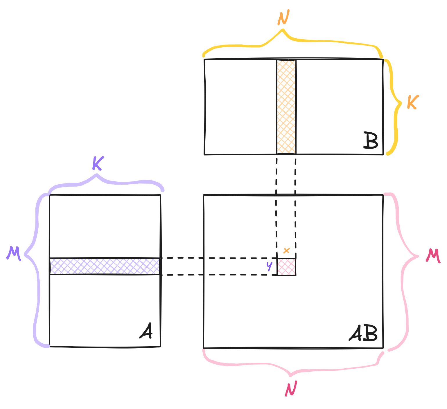
Matrix multiplication between $A$ (dimension: $M \times K$) and $B$ (dimension: $K \times N$), resulting in a matrix with dimension ($M \times N$).

To compute the value of AB[y, x], with $y$ indicating the matrix row and $x$ indicating the matrix column, we perform a dot product between the entire row $y$ of $A$ and the entire column $x$ of $B$:

\[AB[y, x] = \sum_{k=1}^{K} A[y, k] * B[k, x]\]

2. Compute-bound or memory-bound? Introducing the roofline model

In my earlier Reduction (Sum) post, I mentioned that reduction is an example of a memory-bound kernel. But what about GEMM? How can we determine whether it’s compute-bound or memory-bound in the first place? To answer these questions, we’d need to talk about the Roofline Model.

The Roofline Model is designed to guide the optimization process by defining the peak performance achievable on a given hardware. It’s typically visualized as a 2D plot, with Operational Intensity on the $x$-axis and Achievable Throughput on the $y$-axis.

image Roofline model

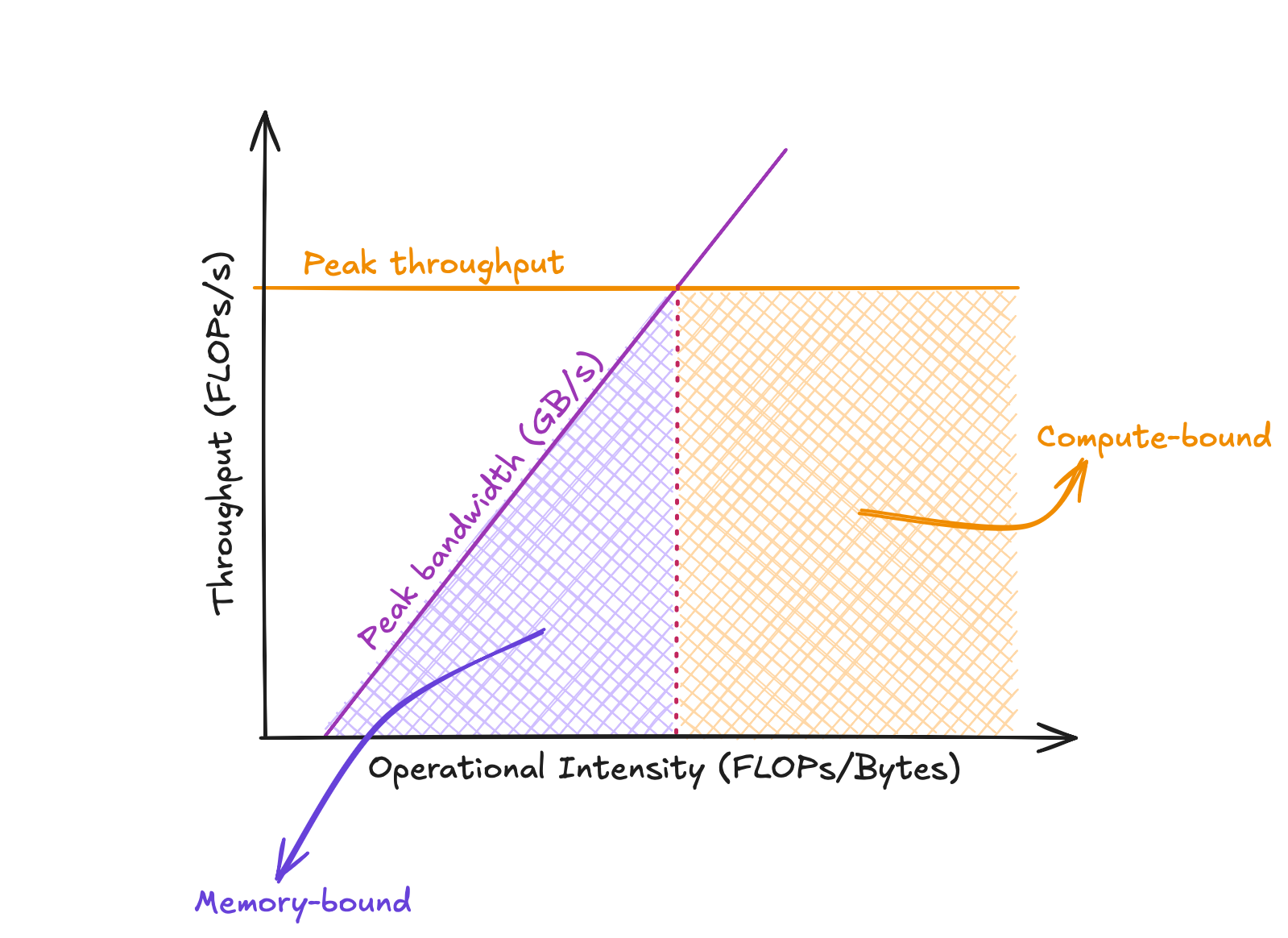
The roofline model.

Operational Intensity measures the number of floating-point operations performed per byte of memory transferred (FLOPs/Bytes).

On the other hand, Throughput, or performance, represents the number of floating-point operations a processor can execute per second (FLOPs/s).

The Roofline Model visualizes two types of “roofs” in a 2D plot:

Memory bandwidth roof, represents the (theoretical) peak memory bandwidth. As noted in the sum reduction post, the RTX 5070 Ti has a peak memory bandwidth of approximately 896 GB/s. This roof appears as a slanted line on the plot, following the equation $Performance = Memory\,Bandwidth \times Operational \, Intensity$.
Compute roof, represents the theoretical peak throughput of the hardware. According to the official specification document, RTX5070Ti achieves a peak FP32 throughput of 43.9 TFLOPs/s for standard floating-point operations, and a peak mixed-precision Tensor Core throughput of 87.9 TFLOPs/s.

Regions below the memory bandwidth roof are considered memory-bound, while regions below the compute roof are considered compute-bound.

Example: determining whether the naive implementation is memory- or compute-bound

Computing the total floating-point operations

To compute the total floating-point operations, we can divide the GEMM operations into 4 steps:

$AB$
For each cell in $C$ (a total of $M \times N$ number of cells), we compute a dot product of $K$ elements from $A$ and $K$ elements from $B$. So we have a total of $(M \times N) \times (K + K - 1)$ FLOPs, where the first $K$ indicates the number of multiplication operations and the latter $K - 1$ indicates the number of addition operations. Note that some references assume the use of fused multiply-add (FMA) instruction, which consists of 1 FLOP of multiply and 1 FLOP of add, simplifying the number of FLOPs to $2 \times M \times N \times K$.
$\alpha AB$
Once we have $AB$ from step 1, we simply run another $MN$ multiplication operations to obtain $\alpha AB$.
$\beta C$
Similar to step 2, we have another $MN$ FLOPs.
$\alpha AB + \beta C$
In our final addition, we perform another $MN$ FLOPs.

To summarize, we have in total of $$ (M \times N) \times (K + K - 1) + 3MN = (2MNK + 2MN) \,FLOPs $$ Computing the total data transferred

Similarly, we can divide the total data transferred into three steps:

$\alpha AB$
For each cell in $C$, we transfer $K$ elements from $A$ and $K$ elements from $B$, so we have in total of $2MNK \times 4\,Bytes$ data transferred.
$\beta C$
We load all elements of $C$ = $MN \times 4\,Bytes$.
$C = \alpha AB + \beta C$ (storing the updated $C$)
We store all elements of $C$ = $MN \times 4\,Bytes$.

Summing the Bytes transferred in all steps, we'll have $$ (2MNK + 2MN) \times 4\,Bytes $$ Computing the operational intensity

Given the total FLOPS and total data transfer calculated above, the operational intensity is only 0.25 FLOPS/Byte. Even if the effective memory bandwidth approaches the peak bandwidth of 896 GB/s on the RTX5070Ti, this corresponds to a theoretical throughput of just 0.224 TFLOPs/s. This value is significantly lower than the GPU's peak non-tensor FP32 performance of 43.9 TFLOPs/s, placing the computation within the memory-bound region of the Roofline Model.

It's important to note that this operational intensity is theoretical. Since elements in $A$ and $B$ are reused across threads and iterations, GPU caches (L1 and L2) automatically serve most repeated accesses; only the first access to a cache line actually goes to DRAM. As a result, Nsight Compute reports a much higher effective operational intensity of 18.33 FLOPs/Byte, because caching hides the majority of DRAM traffic.

Regardless of this difference, the conclusion remains: naive GEMM implementation is memory-bound, and we'll show how optimizing it with different techniques, along with larger $M$, $N$, and $K$ values, shift the performance toward the compute-bound region.

3. Problem setup

We aim to optimize the GEMM operation on matrices $A$, $B$, and $C$ with $M = N = K = 4096$. All matrices are stored in row-major order.

The performance of each kernel is evaluated relative to cuBLAS, which serves as the reference implementation.

4. Single-precision GEMM implementations

In this post, we will look into the following implementations:

Kernel 01: Naive implementation
Kernel 02: Block tiling
Kernel 03: 2D thread coarsening
Kernel 04: Vectorized memory access
Kernel 05: Warp tiling
Kernel 06: Warp tiling, subdivided
Kernel 07: Transposing As
Kernel 08: Asynchronous global-memory loads + double buffering

🚨 CAUTION 🚨

Not all kernels include boundary checks as we ensure that $M$ and $N$ are divisible by the kernel-specific tiling parameters. In practice, however, boundary checks are necessary to prevent incorrect or undefined behavior.

Kernel 01: Naive implementation

image Kernel 01: Naive

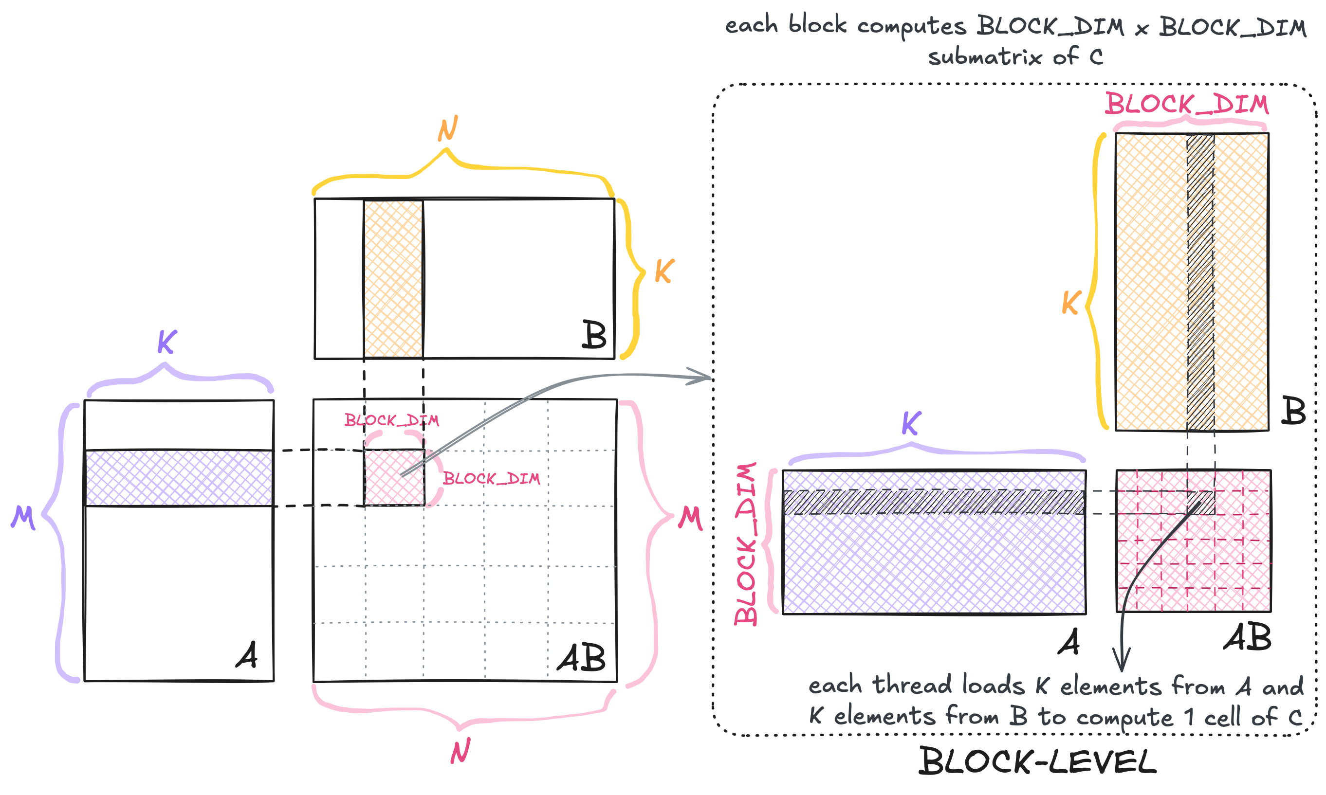
Kernel 01.

In the naive implementation, each BLOCK_DIM x BLOCK_DIM-thread block is responsible for computing BLOCK_DIM x BLOCK_DIM submatrix of $C$. Within each block, every thread loads $K$ elements from $A$ and $K$ elements from $B$, then performs a dot product over these elements. The corresponding kernel code is shown below.

template <uint const BLOCK_DIM>
__global__ void __launch_bounds__(BLOCK_DIM * BLOCK_DIM) naive_gemm(
    int M, int N, int K,
    float alpha,
    float const *__restrict__ A,
    float const *__restrict__ B,
    float beta,
    float *__restrict__ *C
) {
    uint const global_x_idx{blockIdx.x * BLOCK_DIM + threadIdx.x};
    uint const global_y_idx{blockIdx.y * BLOCK_DIM + threadIdx.y};

    // Perform boundary check.
    if (global_x_idx < N && global_y_idx < M) {
        float sum{0.0f};
    
        for (uint k{0}; k < K; ++k) {
            sum += A[global_y_idx * K + k] * B[k * N + global_x_idx];
        }
    
        uint const global_idx{global_y_idx * N + global_x_idx};
        C[global_idx] = alpha * sum + beta * C[global_idx];
    }
}

If You're Curious...

The usages of __launch_bounds__() and __restrict__ are ways to aid optimization by providing additional information to the compiler. More information on __launch_bounds__() and __restrict__ can be found in the CUDA C++ Programming Guide, particularly in sections 10.38. Launch Bounds and 10.2.6. __restrict__, respectively.

Author's Note

If you look at the code, you'd notice that some basic kernel functions have been transformed into function templates so that it can be used for both single- and mixed-precision GEMMs. You can find the list of implemented kernels here.

Note that we use x to represent the horizontal axis and y to represent the vertical axis. This convention helps achieve better memory coalescing behavior:

Threads sharing the same threadIdx.y but having adjacent threadIdx.x values load the same row from $A$. This results in a broadcast rather than true memory coalescing.
Threads with the same threadIdx.y and adjacent threadIdx.x values load adjacent elements from $B$. Because $B$ is stored in row-major order, these accesses are coalesced.

The kernel code can then be invoked using the following host code:

{
    constexpr uint BLOCK_DIM{32};
    assert((N % BLOCK_DIM == 0) && (M % BLOCK_DIM == 0));
    
    dim3 grid_dim(CEIL_DIV(N, BLOCK_DIM), CEIL_DIV(M, BLOCK_DIM));
    dim3 block_dim(BLOCK_DIM, BLOCK_DIM, 1);

    naive_gemm<BLOCK_DIM><<<grid_dim, block_dim>>>(M, N, K, alpha, A, B, beta, C);
}

which yields the following performance:

Kernel #	Performance	% cuBLAS performance
cuBLAS	31.66 TFLOPs/s	100%
kernel 01: naive 🆕	2.05 TFLOPs/s	6.47%

Kernel 02: Block tiling

Recall from Kernel 01 that threads with the same threadIdx.y but different threadIdx.x values in each block load the same row from matrix $A$. Consequently, each element of $A$ is loaded $N$ times, and similarly, each element of $B$ is loaded $M$ times.

One way to reduce global memory traffic is to apply a block tiling technique that leverages shared memory. Since shared memory resides on-chip, it provides a much higher bandwidth than global memory and can lead to a significant improvement in applications with data reuse. One caveat is that shared memory has a much lower capacity compared to global memory; utilizing too much of shared memory can limit the number of blocks that can be scheduled by each SM.

Author's Note

As mentioned in my Reduction post, I highly recommend watching “How CUDA Programming Works” presentation by Stephen Jones. It includes a great explanation and several examples showing how the resources required by each thread block directly affect the number of blocks that can be scheduled on each SM. Shared memory is one such resource to monitor.

Additionally, I’d like to introduce the three stages of the implementation, which I also note as comments in my code:

Shared-memory stores
Dot-product computation
epilogue + output stores

Stage 1 and 2 are carried out within the block tile sliding through $K$, but otherwise, they are independent. For example, I can reuse the shared-memory stores from one kernel and the dot-product computation from another as long as they both follow the same shared-memory layout. Similarly, the epilogue stage is independent of the first two. You may also notice that many optimizations often modify some of the stages, not all.

For each BLOCK_DIM x BLOCK_DIM submatrix (tile) of $C$, the computation in Kernel 02 proceeds as follows.

// Each block allocates two BLOCK_DIM x BLOCK_DIM shared memory buffers:
// one for elements of $A$ (As) and another for elements of $B$ (Bs).

// Each iteration slides the tile to the right in $A$ and downward in $B$ across the $K$ dimension.
for k_offset = 0; k_offset < K; k_offset += BLOCK_DIM {

Stage 1: shared-memory stores

All threads collaboratively store a BLOCK_DIM x BLOCK_DIM tile of $A$ into As corresponding to the same rows as $C$ and columns with range [k_offset, k_offset + BLOCK_DIM).
All threads collaboratively store a BLOCK_DIM x BLOCK_DIM tile of $B$ into Bs corresponding to the same columns as $C$ and rows with range [k_offset, k_offset + BLOCK_DIM).

Stage 2: dot-product computation

Each thread initializes a register sum to store the partial dot product of one cell $c$ in the BLOCK_DIM x BLOCK_DIM submatrix of $C$.
Each thread computes and accumulates the partial dot product into the sum register.

}

Stage 3: epilogue + output stores

Each thread computes $\alpha \times sum + \beta \times c_{value}$ and stores the result back to $C$.

The overall implementation can be illustrated below.

image Kernel 02: Block tiling

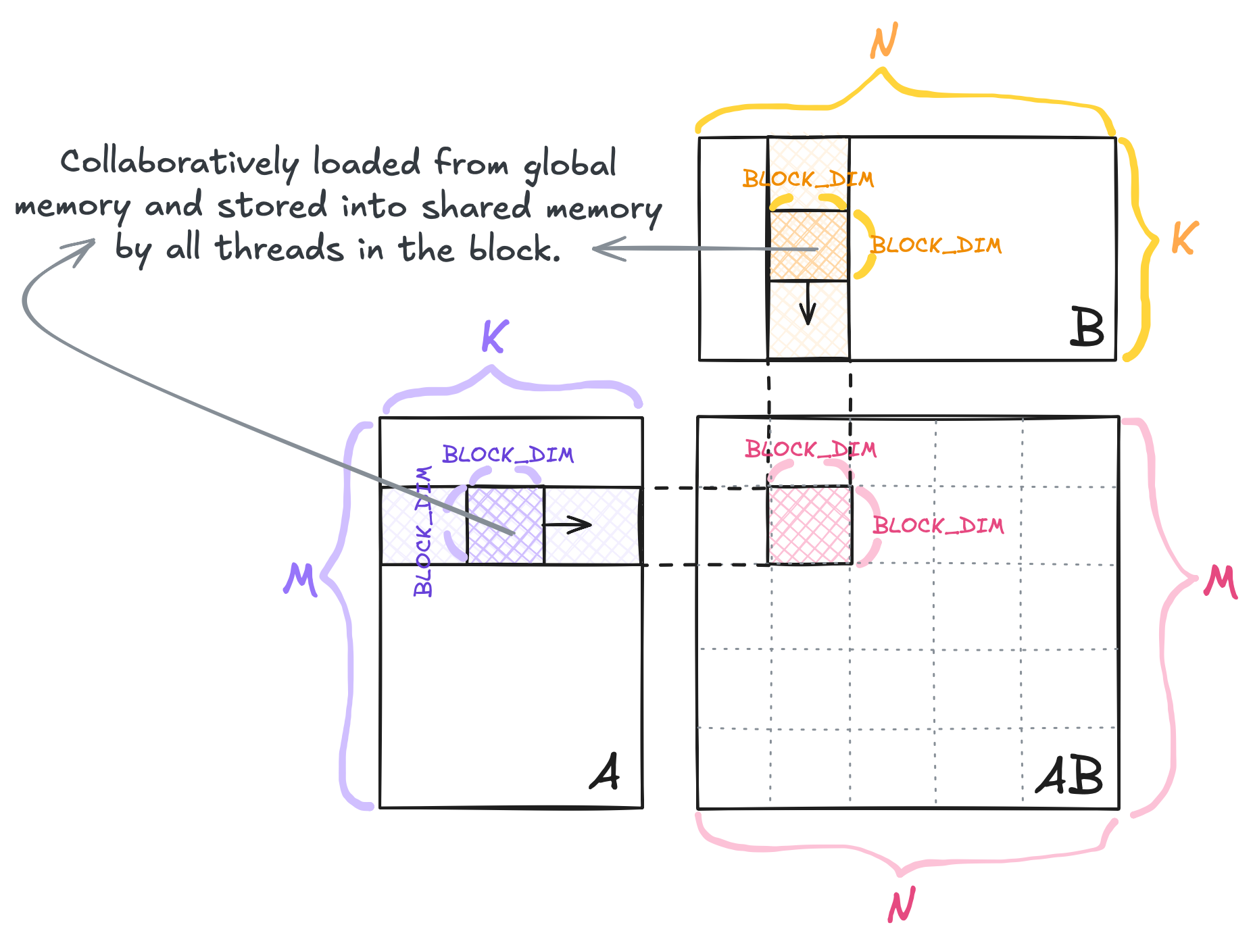
Kernel 02.

And the kernel code is as follows.

template <uint const BLOCK_DIM>
__global__ void __launch_bounds__(BLOCK_DIM * BLOCK_DIM) block_tiling_gemm(
    int M, int N, int K,
    float alpha,
    float const *__restrict__ A,
    float const *__restrict__ B,
    float beta,
    float *__restrict__ C
) {
    __shared__ float As[BLOCK_DIM * BLOCK_DIM];
    __shared__ float Bs[BLOCK_DIM * BLOCK_DIM];

    {
        uint const block_row_offset{blockIdx.y * BLOCK_DIM};
        uint const block_col_offset{blockIdx.x * BLOCK_DIM};

        // Shift A, B, and C with the block offsets.
        A += block_row_offset * K;
        B += block_col_offset;
        C += block_row_offset * N + block_col_offset;
    }

    float sum{0.0f};

    for (uint k_offset{0}; k_offset < K; k_offset += BLOCK_DIM) {
        // Stage 1: shared-memory stores.
        As[threadIdx.y * BLOCK_DIM + threadIdx.x] = A[threadIdx.y * K + threadIdx.x];
        Bs[threadIdx.y * BLOCK_DIM + threadIdx.x] = B[threadIdx.y * N + threadIdx.x];
        __syncthreads();

        A += BLOCK_DIM;
        B += BLOCK_DIM * N;

        // Stage 2: dot-product computation.
        for (uint dot_idx{0}; dot_idx < BLOCK_DIM; ++dot_idx) {
            sum += As[threadIdx.y * BLOCK_DIM + dot_idx] * Bs[dot_idx * BLOCK_DIM + threadIdx.x];
        }
        __syncthreads();
    }

    // Stage 3: epilogue + output stores.
    C[threadIdx.y * N + threadIdx.x] = alpha * sum + beta * C[threadIdx.y * N + threadIdx.x];
}

Author's Note

I found the notion of shifting the pointers difficult to understand at first, so I initially added the offsets within iterations, e.g.,

uint const global_idx{(block_row_offset + threadIdx.y) * N + (block_col_offset + threadIdx.x)};
C[global_idx] = alpha * sum + beta * C[global_idx];

Once I grasped it, while shifting the pointers does simplify the code, I found that adding offsets within loop iterations can sometimes yield noticeably higher throughput.

With the tiling method described above, each element in matrix $A$ in global memory is now accessed only N / BLOCK_DIM times, and each element of matrix $B$ is accessed only M / BLOCK_DIM times. This reduction happens because each BLOCK_DIM x BLOCK_DIM tile is loaded into shared memory once and then reused by all threads in the block, significantly cutting down redundant global memory accesses. As a result, it leads to the following performance increase:

Kernel #	Performance	% cuBLAS performance
cuBLAS	31.66 TFLOPs/s	100%
kernel 01: naive	2.05 TFLOPs/s	6.47%
kernel 02: block tiling 🆕	3.49 TFLOPs/s	11.02%

Kernel 02 in the Roofline Model

Recall that Kernel 02 achieves a throughput of 3.49 TFLOPs/s. The total floating-point operations is the same as Kernel 01, which is $$ 2MN (K + 1) FLOPs $$ The total data transferred, on the other hand, has significantly decreased. Each element in $A$ is now loaded from global memory only N / BLOCK_DIM times, and each element of $B$ is loaded only M / BLOCK_DIM times. Consequently, the total global memory accesses are: $$ A: M \times K \times \frac{N}{BLOCK\_DIM}, \, B: K \times N \times \frac{M}{BLOCK\_DIM} $$ Combined with the global memory access of $C$, the overall global memory traffic becomes: $$ (\frac{2MNK}{BLOCK\_DIM} + 2MN) \times 4 \, Bytes $$ Plugging in $M = N = K = 4096$ and a BLOCK_DIM of $32$, the theoretical operational intensity rises to approximately 7.94 FLOPs/B.

While Kernel 02 remains memory-bound, we can already see a shift from Kernel 01 toward the compute-bound region. To push it further, we need to increase the operational intensity even more. One effective approach is thread coarsening, i.e., allowing each thread to perform more work, which in this case, can further reduce global memory traffic and improve overall performance.

Kernel 03: 2D thread coarsening

This kernel corresponds to Kernel 5 in Simon’s blog post. We now define several new terms:

Block-level
- BM corresponds to the number of rows processed by each block
- BN corresponds to the number of columns processed by each block
- BK contributes to the shared memory size: As uses $BM \times BK$ slots and Bs uses $BK \times BN$ slots.
Thread-level
- TM corresponds to the number of rows processed by each thread
- TN corresponds to the number of columns processed by each thread

The kernel implementation is illustrated below.

image Kernel 01: Naive

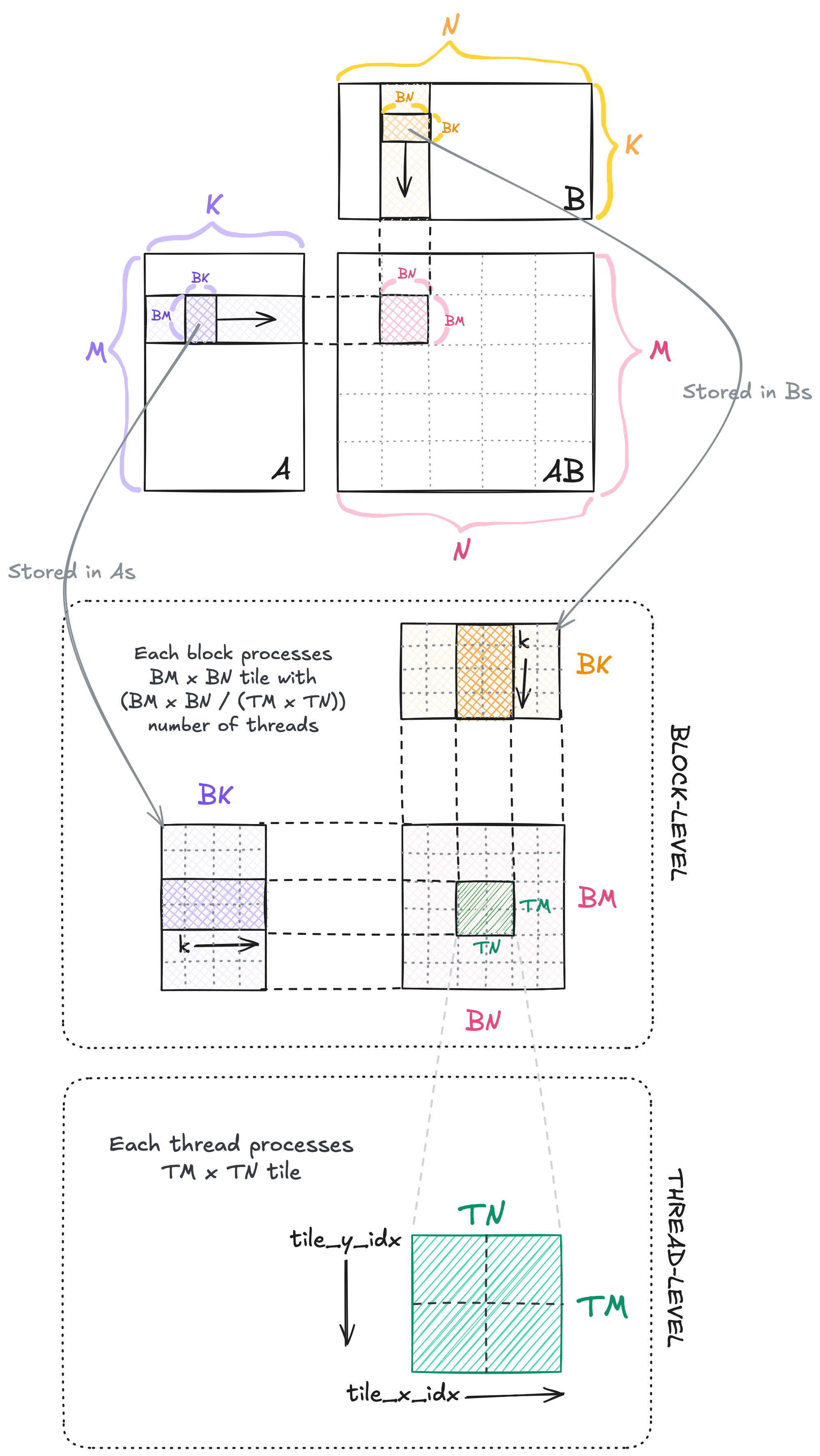
Kernel 03.

This is where I had to remind myself repeatedly that stage 1 (shared-memory stores) and stage 2 (dot-product computation) are independent of each other (my confusion probably stemmed from reusing the same parameter BLOCK_DIM for both the shared-memory stores and the tile size in the previous kernel).

This kernel primarily modifies stage 2 and 3 given the TM x TN tile to process. The only change to stage 1 results from transforming the thread block into one dimension; since the coordinates used in stage 1 and stage 2 (even the thread coordinates for $A$ vs $B$ in stage 2) are now different, it’s easier to work with one-dimensional thread block and generate the coordinates accordingly.

In other words, instead of defining a 2D block shape like this:

dim3 block_dim(BN / TN, BM / TM);

we now switch to a 1D layout:

dim3 block_dim((BM * BN) / (TM * TN));

This simplifies the indexing logic while still covering the same number of threads.

The kernel implementation is as follows.

template <uint const NUM_THREADS, uint const BM, uint const BN, uint const BK, uint const TM, uint const TN>
__global__ void __launch_bounds__(NUM_THREADS) thread_coarsening_2d_gemm(
    int M, int N, int K, float alpha,
    float const *__restrict__ A,
    float const *__restrict__ B,
    float       beta,
    float       *__restrict__ C
) {
    __shared__ float As[BM * BK];
    __shared__ float Bs[BK * BN];

    // CHANGE 1: each thread now computes TM x TN tile.
    float out_values[TM * TN] = {0.0f};

    // CHANGE 2: since the block now has 1D layout, obtain the x and y coordinates
    // within BM x BN (for dot product computation & output stages).
    uint const threadIdx_x{threadIdx.x % (BN / TN)};
    uint const threadIdx_y{threadIdx.x / (BN / TN)};

    ...

    // CHANGE 3.1: compute the number of iterations each thread stores shared memory elements;
    // used only in the shared-memory stores.
    constexpr uint stride_A{NUM_THREADS / BK};
    constexpr uint stride_B{NUM_THREADS / BN};

    // CHANGE 3.2: obtain the row and column indices of A and B during shared-memory stores.
    uint const A_block_row_idx{threadIdx.x / BK};
    uint const A_block_col_idx{threadIdx.x % BK};
    uint const B_block_row_idx{threadIdx.x / BN};
    uint const B_block_col_idx{threadIdx.x % BN};

    for (int k_offset{0}; k_offset < K; k_offset += BK) {
        // Stage 1: shared-memory stores.
        for (int A_load_offset{0}; A_load_offset < BM; A_load_offset += stride_A) {
            As[(A_block_row_idx + A_load_offset) * BK + A_block_col_idx] =
                A[(A_block_row_idx + A_load_offset) * K + A_block_col_idx];
        }
        for (int B_load_offset{0}; B_load_offset < BK; B_load_offset += stride_B) {
            Bs[(B_block_row_idx + B_load_offset) * BN + B_block_col_idx] =
                B[(B_block_row_idx + B_load_offset) * N + B_block_col_idx];
        }
        __syncthreads();

        A += BK;
        B += BK * N;

        // Stage 2: dot-product computation.
        for (int k{0}; k < BK; ++k) {
            for (int tile_y_idx{0}; tile_y_idx < TM; ++tile_y_idx) {
                for (int tile_x_idx{0}; tile_x_idx < TN; ++tile_x_idx) {
                    out_values[tile_y_idx * TN + tile_x_idx] +=
                        As[(threadIdx_y * TM + tile_y_idx) * BK + k] *
                        Bs[k * BN + (threadIdx_x * TN + tile_x_idx)];
                }
            }
        }
        __syncthreads();
    }

    // Stage 3: epilogue + output stores.
    for (int tile_y_idx{0}; tile_y_idx < TM; ++tile_y_idx) {
        for (int tile_x_idx{0}; tile_x_idx < TN; ++tile_x_idx) {
            uint C_idx{};
            {
                uint const cell_row_idx{threadIdx_y * TM + tile_y_idx};
                uint const cell_col_idx{threadIdx_x * TN + tile_x_idx};
                C_idx = cell_row_idx * N + cell_col_idx;
            }
            C[C_idx] =
                alpha * out_values[tile_y_idx * TN + tile_x_idx] +
                beta * C[C_idx];
        }
    }
}

Iterations during shared-memory stores

In many cases, the shared-memory tiles are larger than the number of threads in a block. In other words, BM x BK and BK x BN may exceed the block size. When that happens, each thread must perform multiple iterations to fully populate the shared memory. The strides added in each iteration are defined by stride_A and stride_B, which allow the kernel to loop across BM to fill As and BK to fill Bs. For simplicity, we assume that

(BM x BK) % NUM_THREADS == 0
(BK x BN) % NUM_THREADS == 0
NUM_THREADS % BK == 0
NUM_THREADS % BN == 0

In practice, however, we’ll need proper boundary checks to handle cases where these conditions don’t hold.

The figure below illustrates an example of how stride_A and stride_B are used in loading into shared memory.

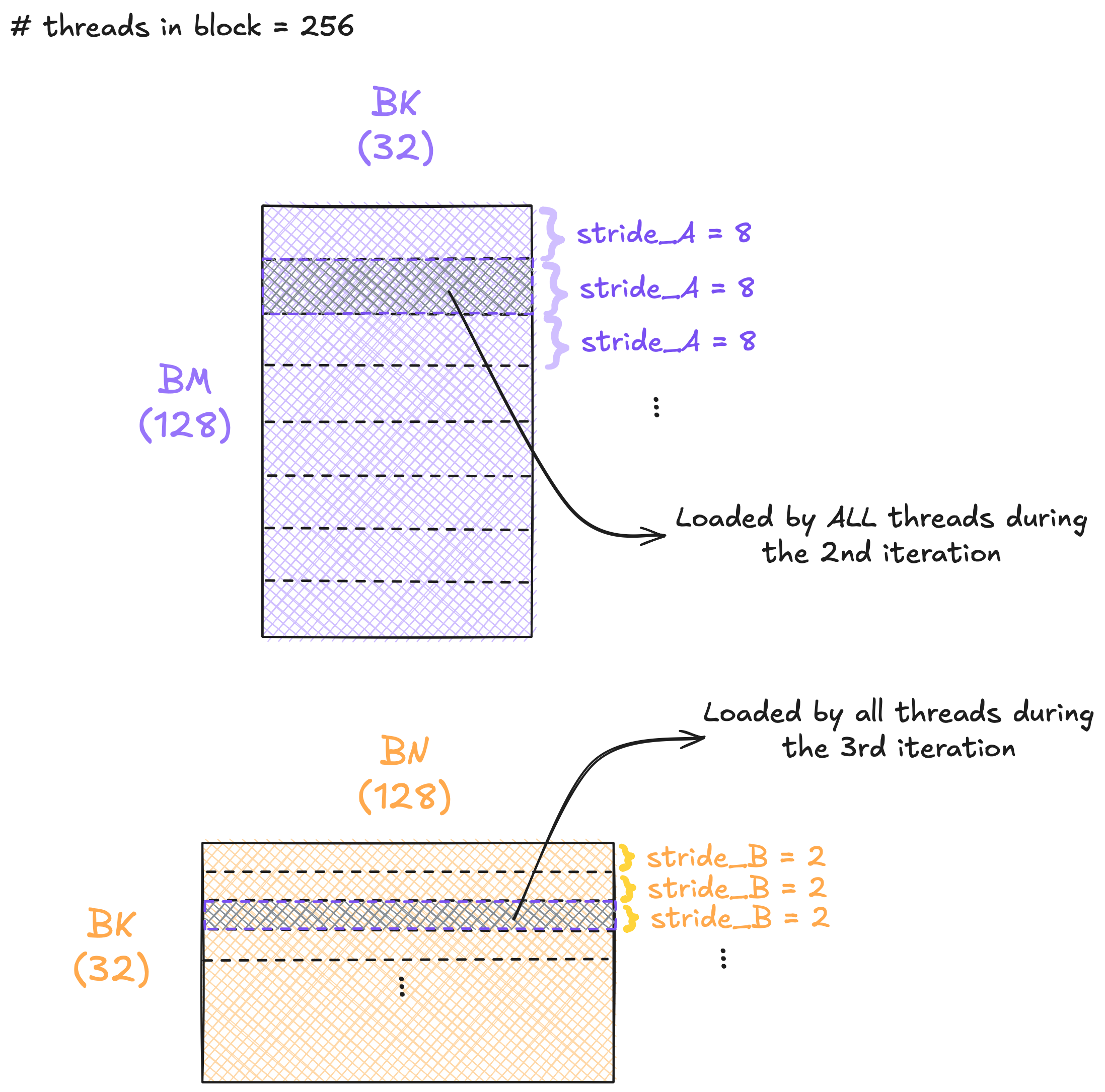
image Shared-memory stores in Kernel 03

An example of shared-memory stores in Kernel 03.

This kernel achieves the following performance, marking a significant jump compared to the previous implementation.

Kernel #	Performance	% cuBLAS performance
cuBLAS	31.66 TFLOPs/s	100%
kernel 01: naive	2.05 TFLOPs/s	6.47%
kernel 02: block tiling	3.49 TFLOPs/s	11.02%
kernel 03: 2D thread coarsening 🆕	20.05 TFLOPs/s	63.33%

Kernel 04: Vectorized memory access

Global memory access is relatively slow, so it’s generally recommended to combine multiple small transfers into a single larger transfer. This approach reduces the overhead associated with each memory access. According to the CUDA C++ Programming Guide, global memory can be accessed using 32-, 64-, or 128-bit memory transactions.

Up to now, all global memory loads have been performed using 32-bit transactions. In Kernel 3, for example, if we inspect the line where elements from A are loaded in Godbolt, we see the PTX instruction: ld.global.f32. The goal of the optimization in this kernel is to reduce the number of global memory transfers by merging them into 128-bit transactions, which improves memory throughput. To do that, we use the built-in vector type float4, which packs four consecutive float elements into a single 16-byte vector.

Additionally, we introduce another level of caching using registers in Stage 2 (dot-product computation). We discussed earlier that shared memory has higher bandwidth compared to global memory. Register access is even faster than shared memory, so since we are reusing elements in shared memory during the TM x TN tile computation, we can store the elements of each column from As and each row from Bs in registers. This technique also helps understanding how matrices are loaded into fragments when using Tensor Cores later.

The code update is as follows.

Stage 1: shared-memory stores

// FACTOR = log2(the number of elements packed together).
// In this case, FACTOR = 2 (4 float elements in float4).
constexpr uint stride_A{(NUM_THREADS << FACTOR) / BK};
constexpr uint stride_B{(NUM_THREADS << FACTOR) / BN};

uint const A_block_row_idx{thread_idx / (BK >> FACTOR)};
uint const A_block_col_idx{(thread_idx % (BK >> FACTOR)) << FACTOR};
uint const B_block_row_idx{thread_idx / (BN >> FACTOR)};
uint const B_block_col_idx{(thread_idx % (BN >> FACTOR)) << FACTOR};

for (int A_load_offset{0}; A_load_offset < BM; A_load_offset += stride_A) {
    // Reinterpret the bit pattern of 4 elements of floats as a float4 element.
    reinterpret_cast<float4 *>(&As[(A_block_row_idx + A_load_offset) * BK + A_block_col_idx])[0] =
        reinterpret_cast<float4 *>(&A[(A_block_row_idx + A_load_offset) * K + A_block_col_idx])[0];
}
    
for (int B_load_offset{0}; B_load_offset < BK; B_load_offset += stride_B) {
    reinterpret_cast<float4 *>(&Bs[(B_block_row_idx + B_load_offset) * BN + B_block_col_idx])[0] =
        reinterpret_cast<float4 *>(&B[(B_block_row_idx + B_load_offset) * N + B_block_col_idx])[0];
}

Stage 2: dot-product computation

This is where the register-level caching is performed.

// Note that the thread offsets have been added to As and Bs.
for (int k{0}; k < BK; ++k) {
    for (int tile_y_idx{0}; tile_y_idx < TM; ++tile_y_idx)
        reg_M[tile_y_idx] = As[tile_y_idx * BK + k];
        
    for (int tile_x_idx{0}; tile_x_idx < TN; ++tile_x_idx)
        reg_N[tile_x_idx] = Bs[k * BN + tile_x_idx];
    
    for (int tile_y_idx{0}; tile_y_idx < TM; ++tile_y_idx) {
        for (int tile_x_idx{0}; tile_x_idx < TN; ++tile_x_idx) {
            out_values[tile_y_idx * TN + tile_x_idx] +=
                reg_M[tile_y_idx] * reg_N[tile_x_idx];
        }
    }
}

Stage 3: epilogue + output stores

for (int tile_y_idx{0}; tile_y_idx < TM; ++tile_y_idx) {
    // Notice that we accumulate tile_x_idx by 4 here.
    for (int tile_x_idx{0}; tile_x_idx < TN; tile_x_idx += 4) {
        uint const cell_row_idx{threadIdx_y * TM + tile_y_idx};
        uint const cell_col_idx{threadIdx_x * TN + tile_x_idx};

        float4 tmp = reinterpret_cast<float4 *>(
            &C[cell_row_idx * N + cell_col_idx]
        )[0];

        tmp.x = alpha * out_values[tile_y_idx * TN + tile_x_idx + 0] + beta * tmp.x;
        tmp.y = alpha * out_values[tile_y_idx * TN + tile_x_idx + 1] + beta * tmp.y;
        tmp.z = alpha * out_values[tile_y_idx * TN + tile_x_idx + 2] + beta * tmp.z;
        tmp.w = alpha * out_values[tile_y_idx * TN + tile_x_idx + 3] + beta * tmp.w;
        reinterpret_cast<float4 *>(
            &C[cell_row_idx * N + cell_col_idx]
        )[0] = tmp;
    }
}

The updated PTX instructions are available in this Godbolt link. Notably, the global memory load/store operations now use ld.global.nc.v4.u32 for $A$ and $B$ memory loads, ld.global.v4.u32 for $C$ memory loads, andst.global.v4.f32 for $C$ memory stores. The shared memory stores, on the other hand, now use st.shared.v4.u32. These changes confirm that the kernel now performs 16-byte (or 128-bit) vectorized memory transfers.

Note that .nc in ld.global.nc.v4.u32 stands for non-coherent cache. It indicates that the global memory being loaded is treated as read-only, i.e., the hardware does not need to maintain immediate coherence with global memory stores across SMs. This allows the GPU to optimize the data-fetch operations. The compiler likely infers that $A$ and $B$ are read-only because there are no global stores to these arrays. We can also increase the likelihood of the compiler detecting read-only data if we use both const and __restrict__; unfortunately, we can’t use const on $A$ and $B$ here since the reinterpret_cast operator cannot cast away const. Read more on how the compiler handles potentially read-only global memory data here.

We now achieve 26.01 TFLOP/s, which is about 80% of the cuBLAS performance!

Kernel #	Performance	% cuBLAS performance
cuBLAS	31.66 TFLOPs/s	100%
kernel 01: naive	2.05 TFLOPs/s	6.47%
kernel 02: block tiling	3.49 TFLOPs/s	11.02%
kernel 03: 2D thread coarsening	20.05 TFLOPs/s	63.33%
kernel 04: vectorized memory access 🆕	26.16 TFLOPs/s	82.63%

Kernel 05: Warp tiling

I initially struggled to understand Simon’s Kernel 10: Warp Tiling, so I started by implementing my own version based on how I interpreted the notion of warp tiling. This process helped me understand how Simon introduces an additional split within the warp to maximize instruction-level parallelism–this is where the thread tiling comes into play as mentioned in the post.

I refer to the non-subdivided warp tiling (i.e., my initial interpretation of warp tiling) as Kernel 5, and the subdivided version (Simon’s warptiling kernel) as Kernel 6.

Threads are always created, scheduled, and executed in groups of 32 called warps. When a multiprocessor receives one or more thread blocks to execute, it splits them into warps, and each warp is managed by the warp scheduler. In a warp tiling kernel, we restructure the work within a warp so that all threads cooperate to compute a tile of $C$, which can further boost performance.

For example, when threads in a warp access contiguous memory addresses, global memory loads can be coalesced, and potential shared-memory bank conflicts become easier to detect and avoid (these conflicts occur when threads in a warp access the same shared memory bank but different addresses; see my Sum Reduction post Kernel 1 for examples).

In Kernel 5, we introduce the following terms:

WM corresponds to the number of rows processed by each warp
WN corresponds to the number of columns processed by each warp

One limitation is that each warp always consists of 32 threads (older GPUs may only have 16 threads per warp). This leads to the following constraints:

The total number of warps per block: NUM_THREADS / 32 = (BM x BN) / (WM x WN)
The total number of threads per warp: 32 = (WM x WN) / (TM x TN)

The following figure illustrates Kernel 05.

Kernel 05

Kernel 05.

Author's Note

I agree with Simon that drawing the illustration helps with understanding the kernel implementation, especially when dealing with more complex methods. While the illustration above is more simplified, I would recommend incorporating $A$ and $B$ (or As and Bs in this case) at each level if things are still unclear, similar to how I illustrate Kernel 04 or how Simon illustrates each kernel.

I ended up drawing the illustrations for Kernel 05 and Kernel 06 so many times on papers while trying to explain the implementation to myself out loud (though I also personally love to draw them; pretty diagrams make me happy 😊).

There is no change to stage 1 (shared-memory stores). You’d notice that I reuse the shared-memory stores function from Kernel 04 in my code.

When it comes to stage 2 (dot-product computation) and stage 3 (epilogue + output stores), aside from the thread-level offsets (e.g., thread row index * TM to get the thread row offset), we now have to consider the warp-level offsets as well. This is done by introducing the following variables:

lane_idx: the index of a thread within its warp, computed as threadIdx.x % 32.
warp_idx: the index of the warp within its block, computed as threadIdx.x / 32.

The warp-level and thread-level offsets can now be computed as follows.

uint const lane_idx{threadIdx.x % 32};
uint const warp_idx{threadIdx.x / 32};

// BN / WN computes the number of warps horizontally.
uint const warp_row_offset{(warp_idx / (BN / WN)) * WM};
uint const warp_col_offset{(warp_idx % (BN / WN)) * WN};

// WN / TN computes the number of thread tiles within a warp horizontally.
uint const thread_row_offset{(lane_idx / (WN / TN)) * TM};
uint const thread_col_offset{(lane_idx % (WN / TN)) * TN};

Once we update the offsets when shifting $A$, $B$, and $C$’s pointers, the rest of the implementation is exactly the same as the previous kernel! That is the beauty of shifting the pointers approach~

Performance-wise, however, we don’t really see much differences between Kernel 04 and Kernel 05:

Kernel #	Performance	% cuBLAS performance
cuBLAS	31.66 TFLOPs/s	100%
kernel 01: naive	2.05 TFLOPs/s	6.47%
kernel 02: block tiling	3.49 TFLOPs/s	11.02%
kernel 03: 2D thread coarsening	20.05 TFLOPs/s	63.33%
kernel 04: vectorized memory access	26.16 TFLOPs/s	82.63%
kernel 05: warp tiling 🆕	26.19 TFLOPs/s	82.72%

Kernel 06: Warp tiling, subdivided

Kernel 05 has the following tiling hierarchy: block tile (BM x BN) --> warp tile (WM x WN) --> thread tile (TM x TN). In Kernel 06, we add another level between warp tile and thread tile. Let’s call the new hierarchy level subwarp tile.

We also introduce some new terms (the same terms used in Simon’s):

WMITER: The number of subwarps within a warp vertically.
WNITER: The number of subwarps within a warp horizontally.
WSUBM: The number of rows within a subwarp, derived from WM / WMITER.
WSUBN: The number of columns within a subwarp, derived from WN / WNITER.

The following figure illustrates the difference between Kernel 05 and Kernel 06.

Kernel 05 vs Kernel 06

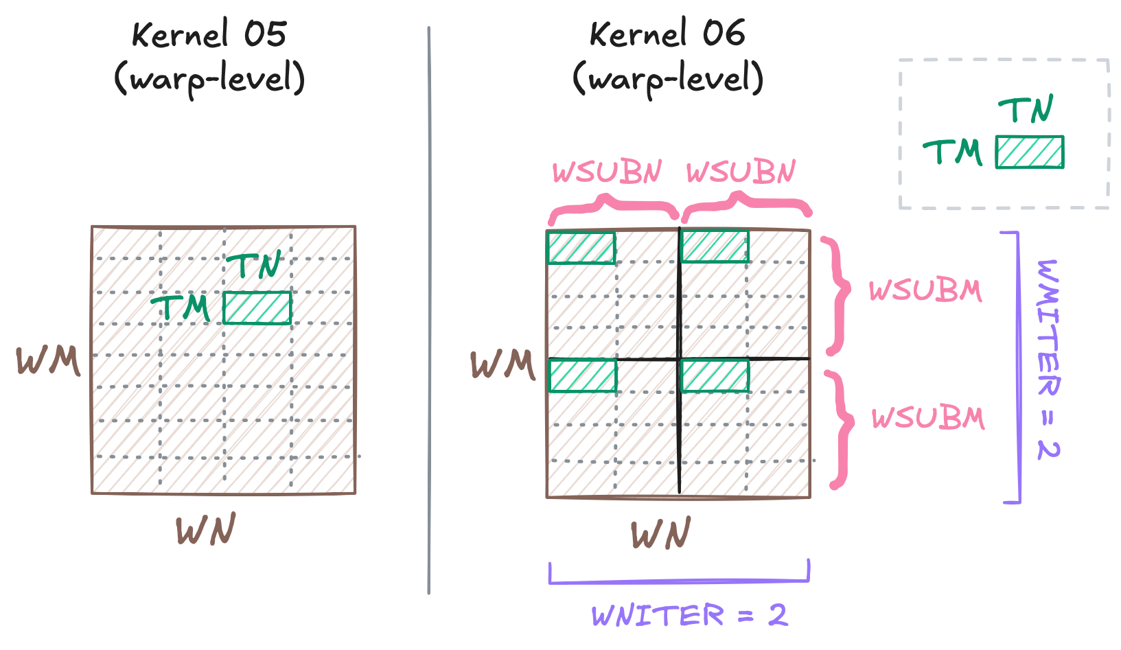
Kernel 05 vs Kernel 06.

Since each warp consists of 32 threads, the following requirement must apply.

\[\frac{WM \times WN}{WMITER \times TM \times WNITER \times TN} = 32\]

Additionally, each thread now computes WMITER * TM * WNITER * TN output elements, compared to only TM * TN output elements in the previous kernel. Some parameter tunings, especially on TM and TN might be necessary.

Stage 1 (shared-memory stores) remains the same as in the previous kernel. In stage 2 (dot-product computation) and stage 3 (epilogue + output stores), we simply place the subwarp loop on top of the existing thread-tiling loop:

Stage 2 (dot-product computation)

// reg_M is now [WMITER * TM] and reg_N is [WNITER * TN].
for (int k{0}; k < BK; ++k) {
    for (int wmiter_idx{0}; wmiter_idx < WMITER; ++wmiter_idx) {
        for (int tm_idx{0}; tm_idx < TM; ++tm_idx) {
            reg_M[wmiter_idx * TM + tm_idx] = As[
                (wmiter_idx * WSUBM + tm_idx) * BK + k
            ];
        }
    }

    for (int wniter_idx{0}; wniter_idx < WNITER; ++wniter_idx) {
        for (int tn_idx{0}; tn_idx < TN; ++tn_idx) {
            reg_N[wniter_idx * TN + tn_idx] = Bs[
                k * BN + (wniter_idx * WSUBN + tn_idx)
            ];
        }
    }

    // out_values is now [WMITER * TM * WNITER * TN].
    for (int wmiter_idx{0}; wmiter_idx < WMITER; ++wmiter_idx)
        for (int wniter_idx{0}; wniter_idx < WNITER; ++wniter_idx)
            for (int tm_idx{0}; tm_idx < TM; ++tm_idx)
                for (int tn_idx{0}; tn_idx < TN; ++tn_idx) {
                    out_values[(wmiter_idx * TM + tm_idx) * (WNITER * TN) + wniter_idx * TN + tn_idx] +=
                        reg_M[wmiter_idx * TM + tm_idx] * reg_N[wniter_idx * TN + tn_idx];
                }
}

Stage 3 (epilogue + output stores)

for (int wmiter_idx{0}; wmiter_idx < WMITER; ++wmiter_idx)
    for (int wniter_idx{0}; wniter_idx < WNITER; ++wniter_idx) {
        uint const tile_row_idx{wmiter_idx * WSUBM};
        uint const tile_col_idx{wniter_idx * WSUBN};
            
        for (int tm_idx{0}; tm_idx < TM; ++tm_idx)
            for (int tn_idx{0}; tn_idx < TN; tn_idx += 4) {
                uint const cell_row_idx{tile_row_idx + tm_idx};
                uint const cell_col_idx{tile_col_idx + tn_idx};
                    
                float4 tmp = reinterpret_cast<float4 *>(
                    &C[cell_row_idx * N + cell_col_idx]
                    )[0];
                uint const first_out_idx = (wmiter_idx * TM + tm_idx) * (WNITER * TN) + wniter_idx * TN + tn_idx;
                tmp.x = alpha * out_values[first_out_idx + 0] + beta * tmp.x;
                tmp.y = alpha * out_values[first_out_idx + 1] + beta * tmp.y;
                tmp.z = alpha * out_values[first_out_idx + 2] + beta * tmp.z;
                tmp.w = alpha * out_values[first_out_idx + 3] + beta * tmp.w;
                reinterpret_cast<float4 *>(
                    &C[cell_row_idx * N + cell_col_idx]
                )[0] = tmp;
            }
    }     

These modifications lead to a performance of 28.70 TFLOPs/s, which is more than 90% of cuBLAS!

Kernel #	Performance	% cuBLAS performance
cuBLAS	31.66 TFLOPs/s	100%
kernel 01: naive	2.05 TFLOPs/s	6.47%
kernel 02: block tiling	3.49 TFLOPs/s	11.02%
kernel 03: 2D thread coarsening	20.05 TFLOPs/s	63.33%
kernel 04: vectorized memory access	26.16 TFLOPs/s	82.63%
kernel 05: warp tiling	26.19 TFLOPs/s	82.72%
kernel 06: warp tiling, subdivided 🆕	28.70 TFLOPs/s	90.65%

How does Kernel 06 lead to such performance improvements?

If we look at my parameters setup, we’ll see that each thread in both Kernel 05 and Kernel 06 compute the same amount of output elements. In particular, each thread computes 128 output elements in both configurations:

Kernel #	NUM_THREADS	WM	WN	TM	TN	WMITER	WNITER
Kernel 05	128	32	128	16	8	1	1
Kernel 06	128	32	128	8	4	2	2

Author's Note

By comparing their configurations side-by-side, I'm suggesting that the Kernel 06 implementation can be reused for Kernel 05 by applying the configuration described above. As a precaution, I ran the Kernel 06 implementation with the Kernel 05 configuration, and it produced performance consistent with the results shown in the performance table.

It’s fascinating to observe that the throughput of Kernel 06 is approximately 10% higher than Kernel 05. One noticeable difference identified when profiling Kernel 05 vs Kernel 06 using Nsight is that Kernel 06 has 12.84% instruction per cycles (IPC) elapsed higher than Kernel 05.

If we examine the PTX instructions for each K iteration in the compute_dot_products() function (where I use Kernel 06 implementation code for both kernels but with different configurations), we can see that increasing both WMITER and WNITER from 1 to 2 changes the ordering of the PTX instructions:

PTX instructions: Kernel 05 vs Kernel 06

PTX instructions: Kernel 05 vs Kernel 06.

The fma (fused multiply-add) instruction can only execute once the data it depends on is already available in registers. In Kernel 05, all eight column values of Bs must be loaded into reg_N (since TN = 8 in the Kernel 05 configuration) before the fma instructions for subsequent rows can be issued. This creates large fma blocks, each containing eight fma instructions. These long dependency chains introduce longer stalls, which reduce instruction-level parallelism (ILP) and ultimately lower IPC.

On the other hand, in Kernel 06, the fma instructions for subsequent rows only need to wait for the first four column elements of Bs to be loaded into reg_N (since TN = 4 in the Kernel 06 configuration). As a result, each fma block is smaller, containing only four fma instructions. After the first TM * TN FMAs complete, we then see the next four reg_N stores begin. Additionally, the PTX instructions in Kernel 06 also include blocks of fully independent FMA instructions with no preceding register loads, which can execute immediately and provide pure ILP, further boosting IPC.

Another way to illustrate the PTX instruction ordering is shown in the diagram below.

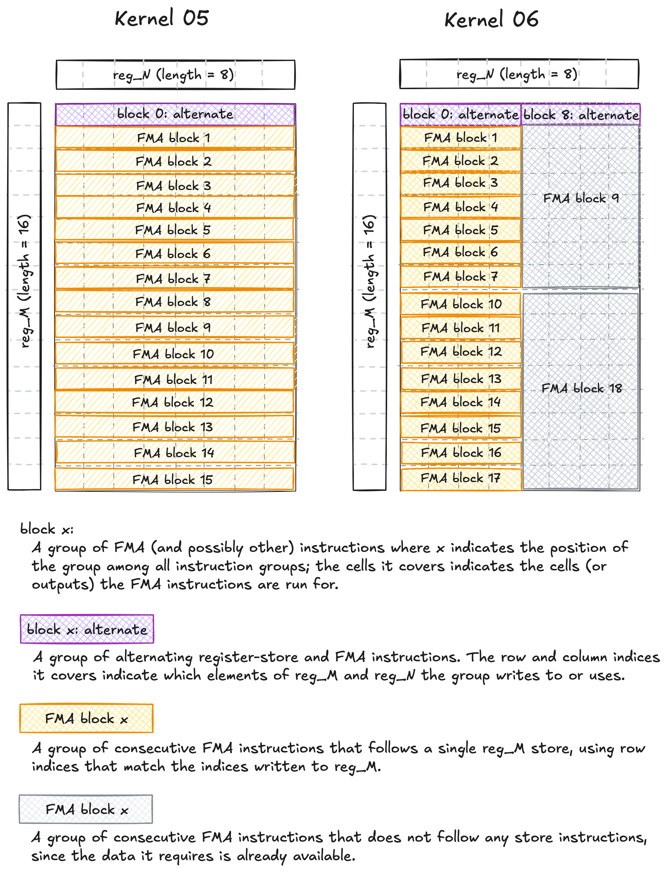
PTX instructions diagram: Kernel 05 vs Kernel 06

PTX instruction diagram: Kernel 05 vs Kernel 06.

Out of curiosity, I experimented with different TM, TN, WMITER, and WNITER configurations while keeping the total number of elements computed per thread the same (i.e., 128 elements). The stage 3 (epilogue + output stores) configuration was kept the same throughout these experiments, which required disabling the matrix verification step temporarily since the different configurations would produce incorrect outputs. Note that TN should always be divisible by 4.

TM	TN	WMITER	WNITER	TFLOPs/s	Remark
8	4	1	4	25.39
8	4	2	2	28.70	Original configuration
8	4	4	1	21.53
4	4	1	8	21.53
4	4	2	4	25.41
4	4	4	2	28.73	Very similar to our original’s performance!
4	4	8	1	21.52
4	8	1	4	21.51
4	8	2	2	22.30
4	8	4	1	26.23
1	16	1	8	15.11
1	16	2	4	19.99
1	16	4	2	15.66
1	16	8	1	15.59

If we group the experiments by TN and look at the the best-performing configuration in each group, we see that larger TN values lead to worse performance. This is expected because a larger TN creates a longer dependency chain: more column elements must be loaded into reg_N before FMAs for subsequent rows can begin.

Focusing on the experiments where TN = 4, we observe that performance increases as WNITER decreases, reaches a peak, and then eventually drops again. When WNITER = 1, there are no blocks of fully independent FMA instructions, which likely explains the performance drop.

However, a larger WNITER does not always guarantee better performance. One possible explanation is that increasing WNITER enlarges the overall block of alternating register-store and FMA instructions. As these blocks grow, they may introduce new dependency chains and ultimately limiting ILP.

Kernel 07: Transposing `As`

One optimization recommended in Simon’s post is to vectorize the shared-memory loads as well. Vectorizing the loads from Bs is straightforward because Bs is always accessed horizontally. In contrast, vectorizing the loads from As requires transposing As since its elements are currenty loaded vertically.

When storing into a transposed As, we can still vectorize the global-memory loads from $A$ using float4, and then manually distribute the four elements into the appropriate rows of the transposed shared-memory buffer:

// Part of load_gmem_to_smem() function.
for (int A_load_offset{0}; A_load_offset < BM; A_load_offset += stride_A) {
    // Keep the vectorized loads.
    float4 tmp = reinterpret_cast<float4 *>(&A[(A_block_row_idx + A_load_offset) * K + A_block_col_idx])[0];

    As[(A_block_col_idx + 0) * BM + A_block_row_idx + A_load_offset] = tmp.x;
    As[(A_block_col_idx + 1) * BM + A_block_row_idx + A_load_offset] = tmp.y;
    As[(A_block_col_idx + 2) * BM + A_block_row_idx + A_load_offset] = tmp.z;
    As[(A_block_col_idx + 3) * BM + A_block_row_idx + A_load_offset] = tmp.w;
}

We then vectorize all shared memory loads as follows.

for (int k{0}; k < BK; ++k) {
    for (int wmiter_idx{0}; wmiter_idx < WMITER; ++wmiter_idx) {
        // Notice that we now add 4 to tm_idx each time.
        for (int tm_idx{0}; tm_idx < TM; tm_idx += 4) {
            reinterpret_cast<float4 *>(&reg_M[wmiter_idx * TM + tm_idx])[0] =
                reinterpret_cast<float4 *>(&As[k * BM + (wmiter_idx * WSUBM + tm_idx)])[0];
        }
    }
    for (int wniter_idx{0}; wniter_idx < WNITER; ++wniter_idx) {
        // Notice that we now add 4 to tn_idx each time.
        for (int tn_idx{0}; tn_idx < TN; tn_idx += 4) {
            reinterpret_cast<float4 *>(&reg_N[wniter_idx * TN + tn_idx])[0] =
                reinterpret_cast<float4 *>(&Bs[k * BN + (wniter_idx * WSUBN + tn_idx)])[0];
        }
    }

    ...

}

After applying these modifications, generating the PTX instructions should now show ld.shared.v4.f32 when loading from shared memory instead of ld.shared.f32.

Overall, transposing As leads to a noticeable improvement compared to Kernel 06!

Kernel #	Performance	% cuBLAS performance
cuBLAS	31.66 TFLOPs/s	100%
kernel 01: naive	2.05 TFLOPs/s	6.47%
kernel 02: block tiling	3.49 TFLOPs/s	11.02%
kernel 03: 2D thread coarsening	20.05 TFLOPs/s	63.33%
kernel 04: vectorized memory access	26.16 TFLOPs/s	82.63%
kernel 05: warp tiling	26.19 TFLOPs/s	82.72%
kernel 06: warp tiling, subdivided	28.70 TFLOPs/s	90.65%
kernel 07: transposing `As` 🆕	29.71 TFLOPs/s	93.84%

Author's Note

I did experiment with only vectorizing Bs loads in Kernel 06. Interestingly, it did not lead to any significant performance improvement.

How does transposing As affect shared memory bank conflicts?

Recall that shared memory is divided into 32 equally-sized banks where each bank can handle a 4-byte load or store operation per clock cycle. Consecutive 4-byte words are assigned to consecutive banks, so in our case, each float element occupies one bank.

Shared memory bank conflicts occur when multiple threads in a warp access different addresses that reside in the same bank. In such cases, the accesses must be serialized, reducing throughput by a factor equal to the number of conflicting requests. An n-way bank conflict means that n distinct memory requests from threads in a warp target the same bank.

As stores

In the previous kernels, each thread-block stores multiple float4 elements loaded from $A$ into a shared-memory buffer As of size $[BM \times BK]$. With my current $BK$ set to 32, elements from the same column but different rows in As are placed in the same bank. Since each thread stores a float4 element, its four float components now occupy four successive banks. In other words, every eight threads together cover all 32 banks. Because a warp contains 32 threads, a warp would cover four consecutive rows, which results in 4-way bank conflicts.

Now that As is transposed, instead of storing into consecutive indices horizontally, we now store the elements into As vertically. The four rows that were initially covered by a warp now become four columns where each column is of size $BK$. Since my $BM$ value is also divisible by 32, i.e., the elements in each column of the transposed buffer are assigned to the same bank, we now have BK-way bank conflicts, which is 32-way bank conflicts in my case…

As loads

How elements in As are initially loaded

The first elements loaded from non-transposed As by all threads in a warp during the kth, WMITER = 0, WNITER = 0 iteration.

In each iteration over K, WMITER, and WNITER, all threads in a warp compute one element from each TM * TN block. As a result, the number of elements a warp needs to load from As equals the number of TM * TN blocks stacked vertically. In my configuration where WM = 32, WMITER = 2, TM = 8, this results in 2-way bank conflicts.

Once As is transposed, the number of elements loaded from As remains the same, but they are now distributed across different columns. Because of this rearrangement, bank conflicts are eliminated.

Summary

With no change to Bs stores and loads, it is interesting to see that although bank conflicts on As appear to be more severe overall in this kernel, vectorizing all shared memory loads and register stores still leads to performance improvements.

Kernel 08: Asynchronous global-memory loads + double buffering

As the name suggests, this kernel applies 2 optimizations:

asynchronous global-memory loads, and
double buffering.

Asynchronous Data Copies (details taken from this presentation)

So far, we have been using synchronous data copies when loading elements from global memory and storing them “directly” into shared memory, e.g., when we run smem[index] = gmem[index]. At the hardware level, however, the data is actually first copied from global memory into registers through the L1 cache, and only then written from registers into shared memory. Consequently, we end up wasting both registers and L1 bandwidth.

Introduced as part of Asynchronous Data Copies in CUDA 11.0, __pipeline_memcpy_async is a memcpy_async primitive that allows data to be copied from global memory to shared memory without passing through registers. Depending on the transfer size, it can even bypass the L1 cache. By avoiding the register path, fewers registers are required, which can in turn improve occupancy.

Global to shared memory copies

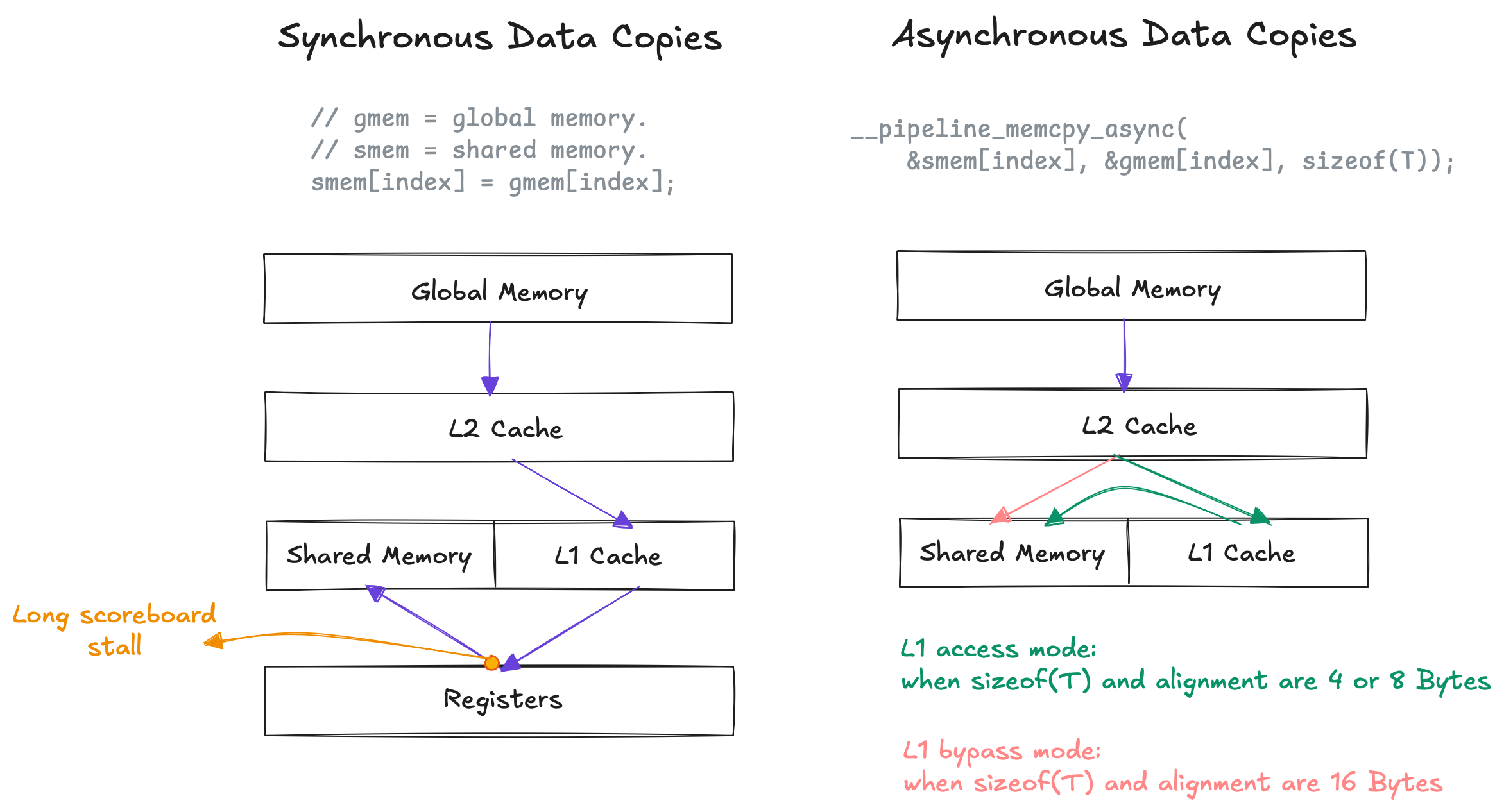
Synchronous vs asynchronous data copies from global to shared memory.

To use asynchronous data copies, we simply replace the stage-1 (shared-memory store) code from Kernel 06 with the code below. We don’t use transposed As here since the current function does not appear to support transposed layouts.

// Make sure to include cuda_pipeline.h.
for (int A_load_offset{0}; A_load_offset < BM; A_load_offset += stride_A) {
    __pipeline_memcpy_async(
        &As[(A_block_row_idx + A_load_offset) * BK + A_block_col_idx],
        &A[(A_block_row_idx + A_load_offset) * K + A_block_col_idx],
        4 * sizeof(float)
    );
}
        
for (int B_load_offset{0}; B_load_offset < BK; B_load_offset += stride_B) {
    __pipeline_memcpy_async(
        &Bs[(B_block_row_idx + B_load_offset) * BN + B_block_col_idx],
        &B[(B_block_row_idx + B_load_offset) * N + B_block_col_idx],
        4 * sizeof(float)
    );
}
__pipeline_commit();

Although not shown here, using the code above might already yield some improvements. We will isolate and examine this improvement in Kernel 10.

Double buffering

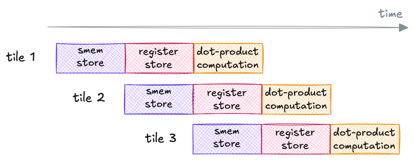
For each sliding tile with length $BK$ across $K$, we currently perform shared-memory stores (stage 1) that is immediately followed by dot-product computation (stage 2) of the particular tile (see the illustration below).

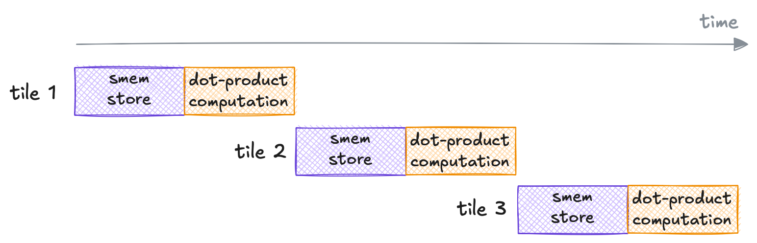
Operation execution timeline of the previous kernels

Operation execution timeline of the previous kernels.

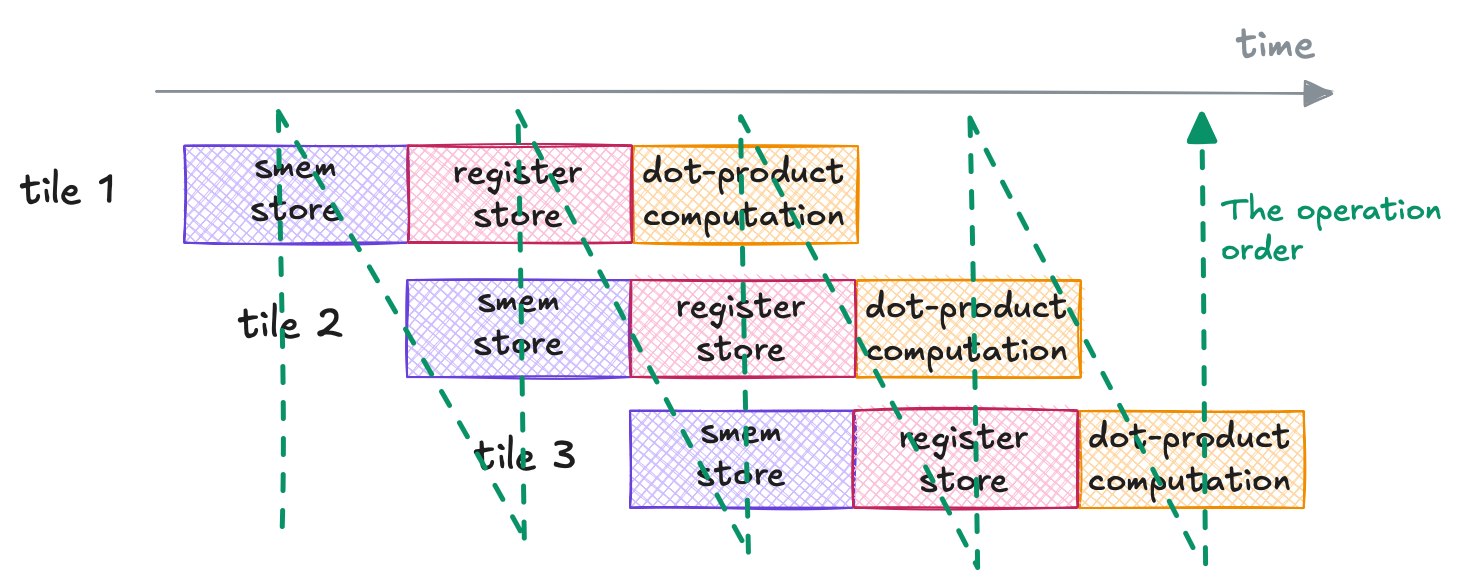
To further hide the data transfer latency, we can overlap the computation with data transfer illustrated as follows.

The new pipeline in Kernel 09

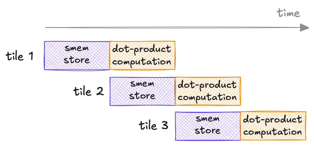
The pipelining approach we aim to use in Kernel 09 to hide data transfer latency.

To enable this, we introduce an additional shared-memory buffer: one buffer holds the data currently used for computation, while the other preloads the next data tile, hence, the name double buffering.

You can find the pseudocode below.

__shared__ float As[2][BM * BK];
__shared__ float Bs[2][BK * BN];

// Load tile 0 elements from A and B into the first buffer of As and Bs.
load_gmem_to_smem(tile[0], A, B, As[0], Bs[0]);

// Define which shared-memory buffer is to be used for computation.
int current{0};

for (tile_index = 1; tile_index < TILE_NUM; ++tile_index) {
    // Load the next tile elements from A and B into the other buffer of As and Bs.
    load_gmem_to_smem(tile[tile_index], A, B, As[current ^ 1], Bs[current ^ 1]);

    // Wait for the second last shared-memory stores to finish (i.e., the current tile).
    __pipeline_wait_prior(1);
    // Make sure all threads have finished loading the current tile.
    __syncthreads();

    // Compute the dot products for the current tile.
    compute_dot_products(As[current], Bs[current], registers, out_values);

    __syncthreads();

    // Update current value.
    current ^= 1;
}

// Wait for the last shared-memory stores to finish.
__pipeline_wait_prior(0);
__syncthreads();
compute_dot_products(As[current], Bs[current], registers, out_values);

// No change.
run_epilogue(...);

Note that I had to scale down the shared-memory usage by reducing $BK$ from 32 to 16, since double buffering requires twice the shared-memory capacity. Keeping BK = 32 would limit the number of blocks that can be scheduled concurrently, which in turn reduces performance instead.

The updated performance table can be found below.

Kernel #	Performance (TFLOPs/s)	% cuBLAS performance
cuBLAS	31.66	100%
kernel 01: naive	2.05	6.47%
kernel 02: block tiling	3.49	11.02%
kernel 03: 2D thread coarsening	20.05	63.33%
kernel 04: vectorized memory access	26.16	82.63%
kernel 05: warp tiling	26.19	82.72%
kernel 06: warp tiling, subdivided	28.70	90.65%
kernel 07: transposing `As`	29.71	93.84%
kernel 08: asynchronous copy + double buffering 🆕	30.28	95.64%

We have now reached beyond 95% of cuBLAS performance on single-precision GEMM!

5. Tensor Cores

Multiply-add is the most frequently used operation in modern neural networks as it is the building block of fully-connected and convolutional layers (read here if you’re curious about how convolutional layers can be mapped into implicit GEMM). As modern neural networks continue to grow in size and demand significantly higher computational capability, the ability to accelerate multiply-add operations becomes crucial.

To address this need, the Volta GPU architecture introduced Tensor Cores, a specialized component of the GPU architecture designed to accelerate matrix multiply-accumulate operations. Tensor Cores provide significantly higher throughput than CUDA cores. For example, on my RTX 5070 Ti, the peak BF16 throughput with FP32 accumulation reaches 87.9 TFLOPs/s, compared to only 43.9 TFLOPs/s of peak non-tensor core FP32 throughput.

There are two ways to use Tensor Cores: via wmma or mma instructions. Both instruction types include load, store, and computation operations, which are performed collectively by all threads in a warp.

wmma instructions can be used through a high-level API or via explicit PTX instructions. Overall, wmma is more straightforward to use, but also more rigid. mma, on the other hand, can only be used via PTX instructions and requires a deeper level of understanding of how it works, but offers greater flexibility. For example, custom swizzling can be used with mma but not with wmma (to my current knowledge; we’ll see a swizzle example with mma in Kernel 14).

Author's Note

Notice two specific details in the explanation above: (1) the emphasis on matrix in matrix multiply-accumulate and (2) the particular example of BF16 throughput with FP32 accumulation.

We will examine these points in more details later, but essentially, Tensor Cores operate on matrices with predetermined sizes and data types for each matrix, depending on the instruction being used (wmma or mma).

6. Mixed-precision GEMM implementations

Tensor Cores do not currently support all data types. The available combinations of data types for the multiplicand and accumulator matrices are listed in this table. For instance, among floating-point data types, there is currently no support for using FP32 for both the multiplicands and the accumulator. Because of that, we will focus on mixed-precision GEMM implementations in the rest of the post.

In particular, we will use the 16-bit alternative floating-point data type BFloat16 (.bf16) for the multiplicands $A$ and $B$, and the 32-bit IEEE floating-point data type (.f32) for the accumulator $C$.

If You're Curious...

BFloat16 stands for Brain Floating Point Format. It is a custom 16-bit floating-point format developed by Google Brain with the goal of accelerating matrix multiplication operations, where each multiply-accumulate operation uses BFloat16 for the multiplication and 32-bit IEEE floating point (FP32) for accumulator.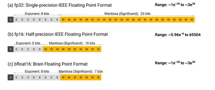

The three floating-point formats; figure taken from the Google Cloud's BFloat16 blog.

As shown in the figure above, BFloat16 has the same dynamic range as FP32 due to having the same number of exponent bits. This allows simpler conversions to and from FP32 compared to FP16 and provides greater robustness against numerical instability during training. Given its 16-bit size, BFloat16 reduces memory usage and can lead to overall faster performance, making it advantageous for layers that do not require a high level of precision. You can read more about the BFloat16 format here.

To implement MP-GEMM, I begin by enabling mixed-precision computation in some of the SGEMM kernels implemented above and examine their performance relative to SGEMM. I then explore the use of Tensor Cores via the wmma APIs and mma instructions, and optimize the implementation from there. Each kernel implementation is compared against the updated cuBLAS performance on MP-GEMM.

The performance of some of the kernels already discussed on mixed-precision GEMM is as follows.

Kernel #	SGEMM Performance (TFLOPs/s)	MP-GEMM Performance (TFLOPs/s)	% MP-GEMM cuBLAS performance
cuBLAS	31.66	88.81	100%
kernel 01: naive	2.05	2.90	3.26%
kernel 02: block tiling	3.49	2.80	3.15%
kernel 04: vectorized memory access	26.16	26.33	29.65%
kernel 05: warp tiling	26.19	26.81	30.19%
kernel 06: warp tiling, subdivided	28.70	27.23	30.66%

While cuBLAS performance shoots up to 88.81 TFLOPs/s for MP-GEMM, kernels up to Kernel 06 show performance similar to SGEMM, so I stopped there and shifted focus to Tensor Cores. I also did not look into why the performance of Kernel 02 dropped in MP-GEMM - perhaps something to look into in the future.

The kernels using Tensor Cores are as follows.

Kernel 09: Tensor Cores (wmma API)
Kernel 10 & 11: Tensor Cores + asynchronous gmem loads + double buffering
Kernel 12: Tensor Cores + three-stage pipeline
Kernel 13: Tensor Cores (mma instructions)
Kernel 14 & 15: Swizzled shared memory + three-stage pipeline

Kernel 09: Tensor Cores (wmma API)

I use the warp matrix functions defined in the namespace nvcuda::wmma in this kernel; I would highly recommend reading the documentation first before continuing reading this post.

To understand how Tensor Cores and the wmma APIs can be used, it helps to visualize and compare the new kernel to Kernel 06 (warptiling, subdivided):

Kernel 06 vs Kernel 09

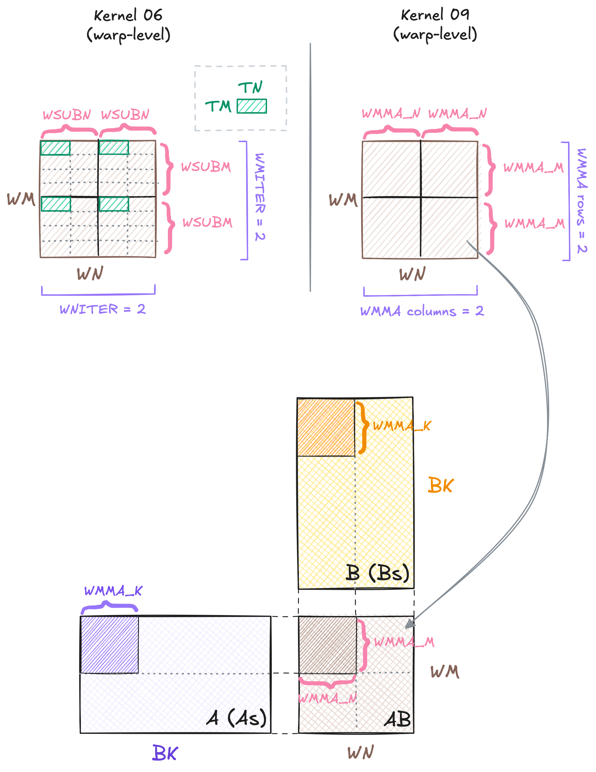
The comparison between Kernel 06 and Kernel 09.

There are three main differences between Kernel 06 and Kernel 09 as illustrated above:

We no longer need to consider the $TM \times TN$ thread tiling explicitly. Although each thread still computes multiple output elements, wmma now determines which threads load data and compute which output elements.
Some changes in terminology:
- WSUBN (or WN / WNITER) becomes WMMA_N
- WSUBM (or WM / WMITER) becomes WMMA_M
In other words, rather than deciding the number of subwarp tiles and deriving the subwarp size, we now choose the subwarp size directly, and the number of subwarp tiles follows.
Kernel 09 introduces WMMA_K, which determines the number of tiles along the $BK$ dimension.

WMMA_M, WMMA_N, and WMMA_K indicate the matrix size; the variety of matrix sizes supported by Tensor Cores are predetermined and can be found here. In the case of using wmma and the BFloat16 data type, the supported matrix sizes are 16x16x16, 32x8x16, and 8x32x16 in the format of mxnxk.

Author's Note

Since there are only three possible matrix sizes, I compared all of them and ultimately chose 16x16x16 for all kernels as it consistently delivers strong performance across the board.

To implement the code, we first create fragments for $A$ and $B$ multiplicands and the accumulator.

// Create fragments.
nvcuda::wmma::fragment<
    nvcuda::wmma::matrix_a, WMMA_M, WMMA_N, WMMA_K, __nv_bfloat16, nvcuda::wmma::row_major> a_frag;
nvcuda::wmma::fragment<
    nvcuda::wmma::matrix_b, WMMA_M, WMMA_N, WMMA_K, __nv_bfloat16, nvcuda::wmma::row_major> b_frag;
nvcuda::wmma::fragment<
    nvcuda::wmma::accumulator, WMMA_M, WMMA_N, WMMA_K, float> acc_frags[NUM_WMMA_M][NUM_WMMA_N];

// Initialize the accumulator fragments.
for (int wmma_row_idx{0}; wmma_row_idx < NUM_WMMA_M; ++wmma_row_idx)
    for (int wmma_col_idx{0}; wmma_col_idx < NUM_WMMA_N; ++wmma_col_idx)
        nvcuda::wmma::fill_fragment(acc_frags[wmma_row_idx][wmma_col_idx], 0.0f);

The usage of Tensor Cores here mainly deals with stage 2 (dot-product computation) and 3 (epilogue + output stores), so there are no changes to stage 1 (shared-memory stores). In this case, I reuse load_gmem_to_smem function from Kernel 04 (vectorized memory access).

Stage 2 (dot-product computation) implementation is as follows.

for (uint wmma_k_offset{0u}; wmma_k_offset < BK; wmma_k_offset += WMMA_K) {
    for (int wmma_row_idx{0}; wmma_row_idx < NUM_WMMA_M; ++wmma_row_idx) {
        // Load from As to a_frag.
        nvcuda::wmma::load_matrix_sync(
            a_frag,
            &As[(wmma_row_idx * WMMA_M) * BK + wmma_k_offset],
            BK
        );

        for (int wmma_col_idx{0}; wmma_col_idx < NUM_WMMA_N; ++wmma_col_idx) {
            // Load from Bs to b_frag.
            nvcuda::wmma::load_matrix_sync(
                b_frag,
                &Bs[wmma_k_offset * BN + (wmma_col_idx * WMMA_N)],
                BN
            );

            // Perform matrix multiplication.
            nvcuda::wmma::mma_sync(
                acc_frags[wmma_row_idx][wmma_col_idx],
                a_frag,
                b_frag,
                acc_frags[wmma_row_idx][wmma_col_idx]
            );
        }
    }
}

As mentioned earlier, we no longer explicitly specify which elements each thread is responsible for. Instead, all threads in a warp collaboratively load elements from As and Bs, store them into the fragments a_frag and b_frag, perform matrix multiplication, and store the results in the corresponding acc_frags tile.

Stage 3 (epilogue + output stores) code can be found below.

// Create a new fragment to hold elements from C.
nvcuda::wmma::fragment<
    nvcuda::wmma::accumulator, WMMA_M, WMMA_N, WMMA_K, float> c_frag;

for (int wmma_row_idx{0}; wmma_row_idx < NUM_WMMA_M; ++wmma_row_idx) {
    for (int wmma_col_idx{0}; wmma_col_idx < NUM_WMMA_N; ++wmma_col_idx) {
        uint const C_row_offset{wmma_row_idx * WMMA_M};
        uint const C_col_offset{wmma_col_idx * WMMA_N};

        nvcuda::wmma::load_matrix_sync(
            c_frag,
            &C[C_row_offset * N + C_col_offset],
            N,
            nvcuda::wmma::mem_row_major
        );

        for (int i{0}; i < c_frag.num_elements; ++i) {
            c_frag.x[i] = alpha * acc_frags[wmma_row_idx][wmma_col_idx].x[i] + beta * c_frag.x[i];
        }

        nvcuda::wmma::store_matrix_sync(
            &C[C_row_offset * N + C_col_offset], c_frag, N, nvcuda::wmma::mem_row_major
        );
    }
}

Notice that the current wmma APIs do not incorporate $\alpha$ and $\beta$, so these must be handled manually. We also cannot simply assume that all fragments are stored in a particular order. For now, the only guarantee is that elements can be mapped safely between fragments of the same type. For example, elements with the same index in different accumulator fragments correspond to the same position in the original matrix, regardless of where that index is stored internally.

If You're Curious...

Unlike wmma, using mma requires understanding the layout of each fragment. Here is an example where we can see the layouts of the multiplicand $A$ fragment, the multiplicand $B$ fragment, and the accumulator fragments in the m16n8k16 matrix for each floating-point data types.

The performance of the kernel can be found in the table below. As we can see, utilizing Tensor Cores significantly improves the throughput to around 70% of cuBLAS performance!

Kernel #	Performance (TFLOPs/s)	% cuBLAS performance
cuBLAS	88.81	100%
kernel 06: warp tiling, subdivided	27.23	30.66%
kernel 09: tensor cores (wmma API) 🆕	65.38	73.62%

Author's Note

If you're still unclear about what fragments are and what they mean for each thread, don't worry! I struggled to understand this as well at the beginning; I only managed to grasp the concept after attempting to use the mma instructions.

We can treat fragments as registers that hold multiple elements. In the m16n8k16 matrix, for instance, 16x16 elements are collectively loaded from As to a_frag by a warp. This means that each thread handles $16 \times 16 / 32 = 8$ elements. So a_frag in each thread contains eight elements, and wmma determines which specific elements each thread is responsible for. Similarly, both b_frag and acc_frag hold four elements each in each thread.

Kernel 10 & 11: Tensor Cores + asynchronous gmem loads + double buffering

In both Kernel 10 and 11, we apply the two optimization techniques from Kernel 08 one by one, specifically:

Kernel 10: we use __pipeline_memcpy_async to bypass registers (and the L1 cache depending on the transfer size) when loading data from global memory into shared memory. Don’t forget to add __pipeline_wait_prior(0) immediately after each global memory load to ensure that all data loads have been completed before resuming with the dot-product computation.
Kernel 11: we overlap computation and shared-memory stores to hide memory latency. To achieve this, we double the shared-memory buffers: one buffer holds the data used by the current computation, while the other holds the data needed for the next computation.

These modifications result in the following performance improvements:

Kernel #	Performance (TFLOPs/s)	% cuBLAS performance
cuBLAS	88.81	100%
kernel 06: warp tiling, subdivided	27.23	30.66%
kernel 09: tensor cores (wmma API)	65.38	73.62%
kernel 10: tensor cores + async gmem loads 🆕	73.77	83.06%
kernel 11: tensor cores + double buffering 🆕	80.33	90.45%

Kernel 12: Tensor Cores + three-stage pipeline

In Kernel 08, we define two levels for overlapping: shared-memory stores and dot-product computation. The dot-product computation itself, however, can be further divided into two steps: (1) register stores and (2) the actual dot-product computation. What if we try overlapping all these three steps, as illustrated below?

Kernel 12 pipeline.

Kernel 12 pipeline.

To do so, we first divide the dot-product computation into the following functions:

1. Loading from shared memory to registers

for (uint wmma_k_idx{0}; wmma_k_idx < NUM_WMMA_K; ++wmma_k_idx) {
    uint const wmma_k_offset{wmma_k_idx * WMMA_K};

    // Load A elements from smem to registers.
    for (int wmma_row_idx{0}; wmma_row_idx < NUM_WMMA_M; ++wmma_row_idx) {
        nvcuda::wmma::load_matrix_sync(
            a_frags[wmma_row_idx][wmma_k_idx],
            &As[(warp_row_offset + wmma_row_idx * WMMA_M) * BK + wmma_k_offset],
            BK
        );
    }

    // Load B elements from smem to registers.
    for (int wmma_col_idx{0}; wmma_col_idx < NUM_WMMA_N; ++wmma_col_idx) {
        nvcuda::wmma::load_matrix_sync(
            b_frags[wmma_k_idx][wmma_col_idx],
            &Bs[wmma_k_offset * BN + (warp_col_offset + wmma_col_idx * WMMA_N)],
            BN
        );
    }
}

2. Run the actual dot-product computation

for (uint wmma_k_idx{0u}; wmma_k_idx < NUM_WMMA_K; ++wmma_k_idx) {
    for (int wmma_row_idx{0}; wmma_row_idx < NUM_WMMA_M; ++wmma_row_idx) {
        for (int wmma_col_idx{0}; wmma_col_idx < NUM_WMMA_N; ++wmma_col_idx) {
            nvcuda::wmma::mma_sync(
                acc_frags[wmma_row_idx][wmma_col_idx],
                a_frags[wmma_row_idx][wmma_k_idx],
                b_frags[wmma_k_idx][wmma_col_idx],
                acc_frags[wmma_row_idx][wmma_col_idx]
            );
        }
    }
}

Since we can no longer directly compute the matrix multiplication, we now need $A$ and $B$ fragments for each WMMA tile.

My first thought of how it overall should be implemented can be illustrated below.

First thought on the order of the operations in Kernel 12

First thought on the order of the operations in Kernel 12.

With the implementation pseudocode below.

load_gmem_to_smem(tile[0], A, B, As[0], Bs[0]); // tile[0].

load_gmem_to_smem(tile[1], A, B, As[1], Bs[1]); // tile[1].

load_smem_to_regs(As[0], Bs[0], A_frags[0], B_frags[0]); // tile[0].

int current{0};

for (tile_index = 2; tile_index < NUM_TILES; ++tile_index) {
    load_gmem_to_smem(tile[tile_index], A, B, As[current], Bs[current]); // tile[2] in 1st iter.

    load_smem_to_regs(As[current ^ 1], Bs[current ^ 1], A_frags[current ^ 1], B_frags[current ^ 1]); // tile[1] in 1st iter.

    compute_dot_products(A_frags[current], B_frags[current], acc_frags); // tile[0] in 1st iter.

    current ^= 1;
}

load_smem_to_regs(As[current ^ 1], Bs[current ^ 1], A_frags[current ^ 1], B_frags[current ^ 1]); // last tile.

compute_dot_products(A_frags[current], B_frags[current], acc_frags); // second last tile.

compute_dot_products(A_frags[current ^ 1], B_frags[current ^ 1], acc_frags); // last tile.

// No change.
run_epilogue(...);

Recall that we now have $A$ and $B$ fragments for each WMMA tile. Given the implementation above, we would also need two buffers for each multiplicand fragment, just like how we allocate two buffers for the shared memory. Because of this, we end up with significantly more registers per thread, which further reduces both the occupancy and the performance in my case.

Fortunately, we can actually switch the order of the operations within the loop such that we no longer need the second buffer for the fragments. The key observation is that it is not necessary to perform the register stores for the next computation before carrying out the dot-product computation for the current one! So within the for loop, we can actually do the following ordering:

for (tile_index = 2; tile_index < NUM_TILES; ++tile_index) {
    load_gmem_to_smem(tile[tile_index], A, B, As[current], Bs[current]); // tile[2] in 1st iter.

    compute_dot_products(A_frags, B_frags, acc_frags); // tile[0] in 1st iter.

    // A_frags and B_frags are now free to use, so we can reuse it in the register stores!
    load_smem_to_regs(As[current ^ 1], Bs[current ^ 1], A_frags, B_frags); // tile[1] in 1st iter.

    current ^= 1;
}

Similarly, we run the dot-product computation first after the for loop ends.

compute_dot_products(A_frags, B_frags, acc_frags); // second last tile.

load_smem_to_regs(As[current ^ 1], Bs[current ^ 1], A_frags, B_frags); // last tile.

compute_dot_products(A_frags, B_frags, acc_frags); // last tile.

With these modifications, we’re able to keep register usage sufficiently low and reach 98% of cuBLAS performance!

Kernel #	Performance (TFLOPs/s)	% cuBLAS performance
cuBLAS	88.81	100%
kernel 01: naive	2.90	3.26%
kernel 02: block tiling	2.80	3.15%
kernel 04: vectorized memory access	26.33	29.65%
kernel 05: warp tiling	26.81	30.19%
kernel 06: warp tiling, subdivided	27.23	30.66%
kernel 09: tensor cores (wmma API)	65.38	73.62%
kernel 10: tensor cores + async gmem loads	73.77	83.06%
kernel 11: tensor cores + double buffering	80.33	90.45%
kernel 12: tensor cores + three-stage pipeline 🆕	87.13	98.11%

Kernel 13: Tensor Cores (mma instructions)

So far, our kernels have mainly relied on the wmma APIs. When loading the matrices into registers using these APIs (i.e., calling load_matrix_sync()), we can only provide the starting address, the stride in elements between consecutive rows or columns depending on the layout, and the memory layout of the matrix. The API then implicitly determines how the data is distributed across threads in the warp.

In some situations, however, we need greater flexibility in how individual threads interact with matrix fragments. Achieving this level of flexibility requires using the low-level MMA instructions directly.

As mentioned earlier, working with mma instructions demands a much deeper understanding of their underlying mechanics. We will walk through the implementation step-by-step.

Note that the matrix sizes supported by wmma and mma are different. When using BFloat16 as multiplicands, mma supports only the m16n8k16 and m16n8k8 shapes. In the remaining kernels, we’ll use the m16n8k16 matrix size.

If You're Curious...

If you're wondering why wmma and mma have different supported matrix sizes, someone also asked the same question here.

Just like Kernel 09, there’s no change to stage 1 (shared-memory stores). We will cover the modifications in stage 2 and stage 3, particularly:

Storing elements into $A$ and $B$ fragments,
Performing matrix multiplication, and
Epilogue and output stores

1. Storing elements into $A$ and $B$ fragments

The ldmatrix instruction is used to load matrix elements from shared memory into fragment registers. In this process, threads can have two roles:

some or all threads supply the shared-memory addresses from which the matrix elements are loaded
all threads allocate and provide the destination registers that receive the loaded elements

Before we discuss this further, let’s start with examining the syntax of the instruction.

ldmatrix.sync.aligned.shape.num{.trans}{.ss}.type r, [p];

.shape   = {.m8n8, .m16n16};
.num     = {.x1, .x2, .x4};
.ss      = {.shared{::cta}};
.type    = {.b16, .b8};

When performing the instruction, all threads in a warp collectively load a matrix from the location indicated by address operand p in the specified state space .ss into destination register r. In our case, .ss and .type are simply .shared and .b16, respectively.

To determine the correct value for the remaining parameters and arguments, we need to consider the following key aspects:

The values of .shape. and .num are based on the data type and the chosen matrix size

Since we are loading 16-bit data, we must use .m8n8 matrix load as it is the only matrix load shape that supports 16-bit data types. The .shape parameter and the matrix size we choose then determine the .num parameter. In the case of choosing the m16n8k16 matrix size, we load a 16x16 matrix from As into $A$ fragment registers, which is four .m8n8 matrix loads. We then load a 16x8 matrix from Bs into $B$ fragment registers, which is two .m8n8 matrix loads. So .num when loading into $A$ and $B$ fragments are .x4 and .x2, respectively.

In some situations, not all threads are responsible for providing the values of .p

Depending on the value of .num, every group of eight threads provides eight addresses where each address corresponds to the start of a matrix row (see the following table; we’ll look into what “matrix rows” mean in the next key point). For example, if .num is .x2, only the first 16 threads in a warp provide addresses 0 - 15. Based on my experience, it seems that the instruction would just ignore whatever addresses passed by the rest of the threads.

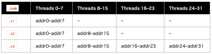
The addresses provided by the corresponding groups of threads in ldmatrix.

The addresses provided by the corresponding groups of threads in ldmatrix; table taken from PTX ISA documentation.

The shared memory addresses p the participating threads need to supply are based on the layout of the fragments

How one or more .m8n8 matrix loads are arranged relative to one another determines the address that each participating thread needs to provide. For example, the arrangement of four .m8n8 matrix loads for 16x16 $A$ fragment and two .m8n8 matrix loads for 16x8 $B$ fragment are illustrated below.

A fragment layout

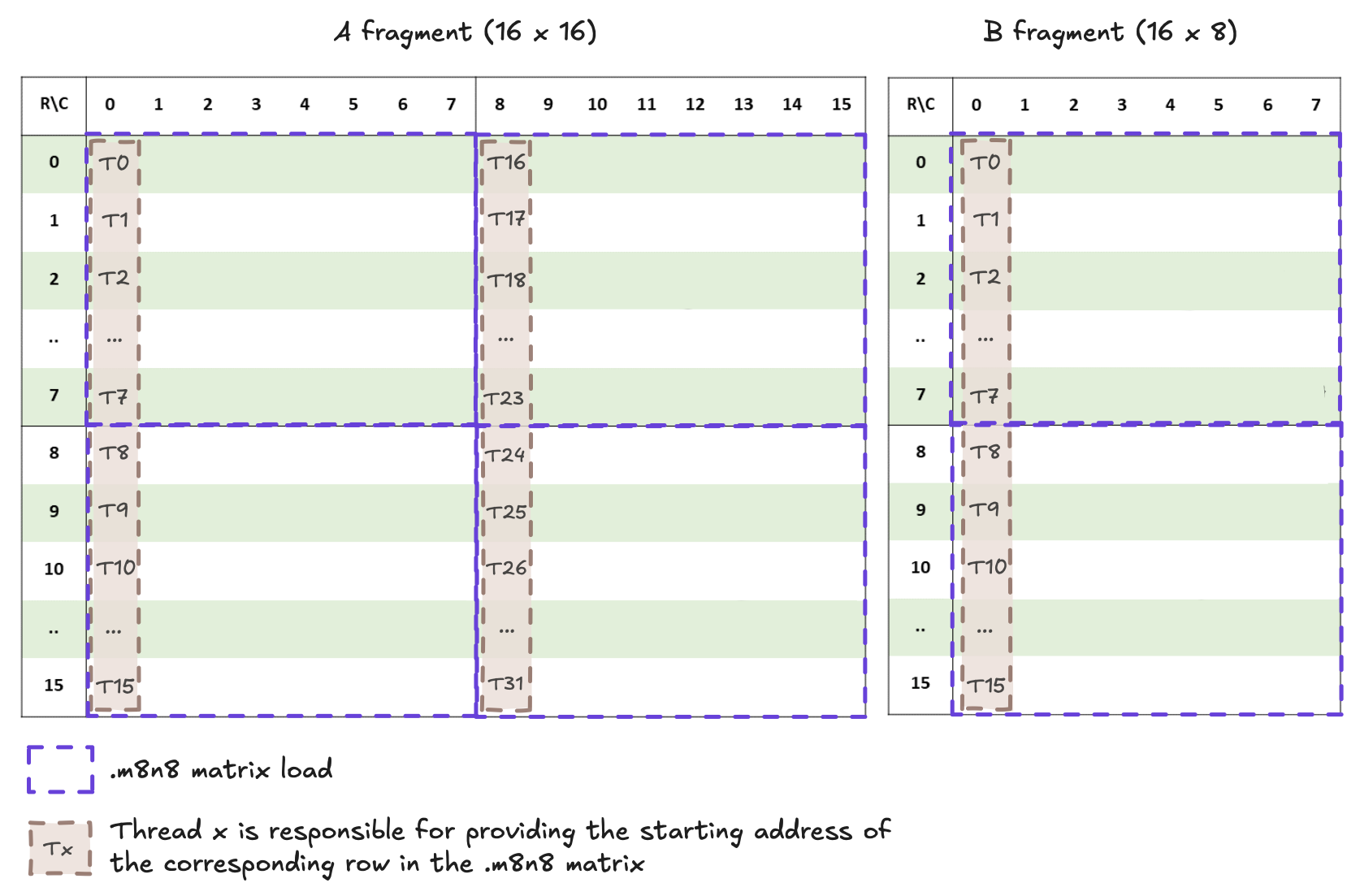
$A$ fragment layout.

The starting address of each row in As can then be computed as follows.

// Note that in the Github code, the computations below are combined.
As_mma_tile_row_offset = warp_row_offset + mma_row_idx * MMA_M;
As_mma_tile_col_offset = mma_k_offset;

As_fragment_row_idx = lane_idx % MMA_M; // MMA_M is 16 in m16n8k16.
As_fragment_col_idx = (lane_idx / MMA_M) * 8; 

As_starting_address_row_idx = As_mma_tile_row_offset + As_fragment_row_idx;
As_starting_address_col_idx = As_mma_tile_col_offset + As_fragment_col_idx;

Note that since the state space of the address is .shared, the 64-bit (generic) CUDA C++ pointer to As will need to be converted into the 32-bit PTX shared state space, hence, the following code is added:

uint32_t shared_A_pointer = static_cast<uint32_t>(
    __cvta_generic_to_shared(&As[As_starting_address_row_idx * BK + As_starting_address_col_idx]));

Similarly, the pointer to Bs can be computed as follows.

// Note that in the Github code, the computations below are combined.
Bs_mma_tile_row_offset = mma_k_offset;
Bs_mma_tile_col_offset = warp_col_offset + mma_col_idx * MMA_N;

Bs_fragment_row_idx = lane_idx % MMA_K;
Bs_fragment_col_idx = 0; // Only one .8x8 matrix is loaded horizontally.

Bs_starting_address_row_idx = Bs_mma_tile_row_offset + Bs_fragment_row_idx;
Bs_starting_address_col_idx = Bs_mma_tile_col_offset + Bs_fragment_col_idx;

uint32_t shared_B_pointer = static_cast<uint32_t>(
    __cvta_generic_to_shared(&Bs[Bs_starting_address_row_idx * BN + Bs_starting_address_col_idx]));

All threads need to allocate and provide destination registers r

Unlike how we can use the fragment class in wmma, we need to create our own fragment registers when using mma directly. The number of elements each thread needs to store in the $A$ and $B$ fragment registers is listed in the PTX ISA documentation.

According to the documentation for BFloat16-based m16n8k16 matrix, the multiplicand $A$ fragment holds “four .f16x2 registers, with each register containing two .bf16 elements from the matrix $A$”. An initial approach, therefore, would be to define the following registers:

__nv_bfloat16 A_register[8];

However, the CUDA device compiler does not automatically pack two 16-bit data types into a single 32-bit register. So to ensure that the 16-bit .bf16 elements are packed consecutively, we use 32-bit-based registers instead:

// We now need 8 * 16 / 32 = 4 elements per 32-bit register.
uint32_t A_register[4];

Using the same approach, we define the following $B$ fragment registers:

uint32_t B_register[2];

We then can pass these registers as destination registers in the ldmatrix instruction.

Which registers hold which elements in the fragment matrix? This is where the fragment layouts shown in the PTX ISA documentation come into place. Let’s look at the m16n8k16 matrix $A$ fragment layout.

A fragment layout

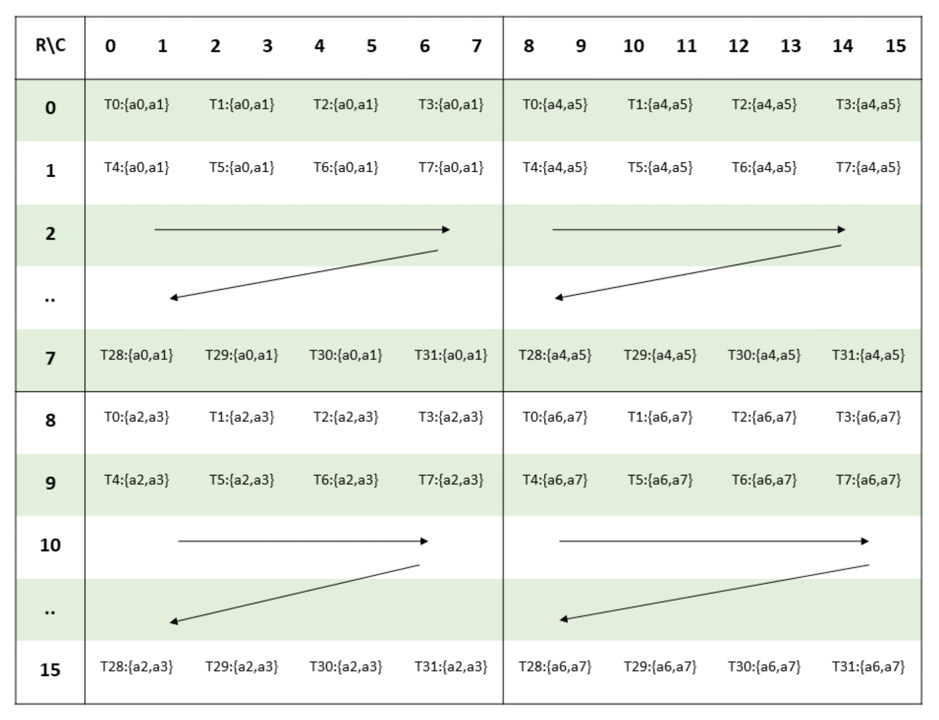
$A$ fragment layout for m16n8k16 matrix size.

As we can see from the figure above, each thread holds eight .bf16 elements, with every two .bf16 elements packed into a single .bf16x2 register. For instance, thread 0 stores the elements at coordinates [[0, 0], [0, 1], [8, 0], [8, 1], [0, 8], [0, 9], [8, 8], [8, 9]].

The packing and distribution of these elements are handled automatically by ldmatrix. For example, if we specify "=r"(A_register[0]), "=r"(A_register[1]), "=r"(A_register[2]), "=r"(A_register[3]) as the destination registers, then A_register[0] will hold values a0 and a1, A_register[1] will hold a2 and a3, A_register[2] will hold a4 and a5, and A_register[3] will hold a6 and a7.

We then repeat the same process for the $B$ fragment. The only additional detail is the .trans modifier, which transposes the matrix during loading since the $B$ fragment is stored in column-major order.

Summary

Overall, we’ll have the following instruction:

ldmatrix instruction

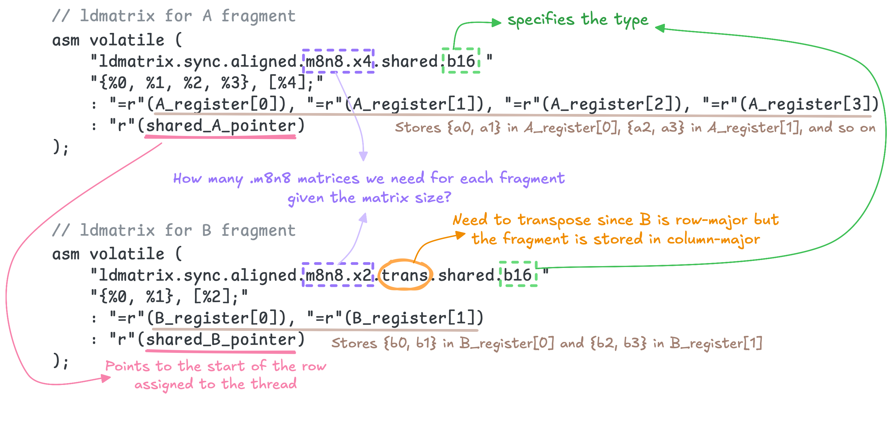
The final ldmatrix instructions for m16n8k16 matrix size with BFloat16 data types.

2. Performing matrix multiplication

We’ve now gotten passed the most complicated part (at least in my opinion, ldmatrix is the most complex instruction to understand!).

Performing matrix multiplication for our problem is pretty straightforward. We simply use mma.sync and pass along our registers:

mma.sync instruction

The mma.sync instruction for m16n8k16 matrix size with BFloat16 data types.

And that’s it!

3. Epilogue and output stores

As with the wmma APIs, we need to apply $\alpha$ and $\beta$ manually here as well. At this stage, acc_frag already contains the accumulated dot products produced by mma.sync. All that remains is to extract the values from acc_frag, load the corresponding values from $C$, perform the final computation, and write the results back to $C$.

Note that we can’t use ldmatrix or stmatrix here since both instructions currently do not support 32-bit data transfer.

We need to pay close attention to the layout of elements within the accumulator fragment here.

Accumulator fragment layout

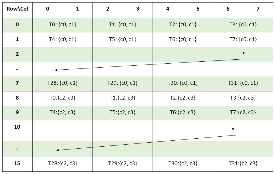
The accumulator fragment layout for m16n8k16 matrix size.

Based on the layout shown above, each thread holds four .f32 elements, with every two elements grouped and stored consecutively. To obtain the corresponding fragment row and column indices for each thread, we can compute them as shown in the following code. Since the elements are already paired, we can also vectorize the loads and stores using float2.

uint const fragment_row_offset{lane_idx / 4};
uint const fragment_col_offset{(lane_idx % 4) * 2};

The rest of the code should be straightforward:

// Load elements from C.
reinterpret_cast<float2 *>(&C_register[0])[0] =
    reinterpret_cast<float2 *>(&C_pointer[fragment_row_offset * N + fragment_col_offset])[0];
reinterpret_cast<float2 *>(&C_register[2])[0] =
    reinterpret_cast<float2 *>(&C_pointer[(fragment_row_offset + 8) * N + fragment_col_offset])[0];

// Compute alpha * (AB) + beta * C.
C_register[0] = acc_register[mma_row_idx][mma_col_idx][0] * alpha + C_register[0] * beta;
C_register[1] = acc_register[mma_row_idx][mma_col_idx][1] * alpha + C_register[1] * beta;
C_register[2] = acc_register[mma_row_idx][mma_col_idx][2] * alpha + C_register[2] * beta;
C_register[3] = acc_register[mma_row_idx][mma_col_idx][3] * alpha + C_register[3] * beta;

// Store outputs back to C.
reinterpret_cast<float2 *>(&C_pointer[fragment_row_offset * N + fragment_col_offset])[0] =
    reinterpret_cast<float2 *>(&C_register[0])[0];
reinterpret_cast<float2 *>(&C_pointer[(fragment_row_offset + 8) * N + fragment_col_offset])[0] =
    reinterpret_cast<float2 *>(&C_register[2])[0];

Unfortunately, we can’t directly compare the performance with Kernel 09 given the different supported matrix sizes. But using mma instructions along with shared-memory stores from Kernel 10 already yields a promising throughput of 76.93 TFLOPs/s.

Kernel #	Performance (TFLOPs/s)	% cuBLAS performance
cuBLAS	88.81	100%
kernel 06: warp tiling, subdivided	27.23	30.66%
kernel 09: tensor cores (wmma API)	65.38	73.62%
kernel 10: tensor cores + async gmem loads	73.77	83.06%
kernel 11: tensor cores + double buffering	80.33	90.45%
kernel 12: tensor cores + three-stage pipeline	87.13	98.11%
kernel 13: tensor cores (mma) 🆕	76.93	86.62%

Author's Note

You can read the Using Inline PTX Assembly in CUDA documentation to become more familiar with the syntax and related details.

Kernel 14 & 15: Swizzled shared memory + three-stage pipeline

We touched on shared memory bank conflicts briefly when implementing Kernel 07 (transposing As). As a reminder:

Shared memory is divided into 32 equally-sized banks, each bank can handle one 4-byte load or store operation per clock cycle. In our case, two consecutive BFloat16 elements share a single bank.
Bank conflicts happen when multiple threads in a warp access different 32-bit locations within the same bank in a single instruction.
- The broadcast rule applies when multiple threads request for the same 32-bit location in that bank. In other words, if one thread requests the first 16 bits and another requests the next 16 bits within the 32-bit location in a bank, no bank conflict occurs (source).
An n-way bank conflict reduces throughput by a factor of n, so we want to minimize them whenever possible.
In some cases, it may not be possible to eliminate all bank conflicts; we will see examples of this in this section.

Bank conflicts often occur because the number of columns in shared memory is usually a multiple of 32 and we typically want to access the elements within the same column. One way to reduce these conflicts is to permute the elements in each row so that consecutive accesses no longer target the same bank. This technique is known as shared memory swizzling. In this post, we will cover the swizzle method from CUTLASS.

The swizzle method from CUTLASS has only three parameters:

BBits –> the number of bits in the bit mask. The mask is created as (1 << BBits) - 1. For example, BBits = 3 would produce a bit mask of ..00111.
MBase –> the number of least significant bits we want to keep constant. This is useful when a group of elements must stay together and the order of the elements within the group always remain the same.
SShift –> the distance to shift right the YYY mask. YYY mask is defined as yyy_mask = bit_mask << (MBase + SShift). For simplicity, we only consider positive values of SShift.

Given an offset (or an index to permute), we perform the following operation:

Swizzle operation from CUTLASS

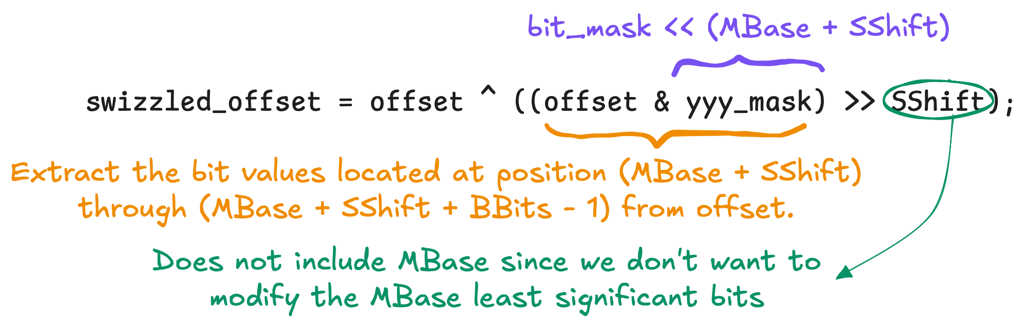
Swizzle operation from CUTLASS.

How do we determine the values of the parameters?

The value of MBase is determined by:

\[log_{2}(number\ of\ elements\ that\ must\ stay\ together).\]

For example, when vectorizing loads or stores of 2-byte elements using a float4, we need to keep eight elements contiguous. In this case, MBase$= log_{2}(8) = 3$. As another example, when using ldmatrix to load fragments, MBase is set to $log_{2}(8) = 3$ since each .m8n8 matrix row contains 8 elements.

BBits is defined as

\[log_{2}(number\ of\ elements\ (or\ groups\ of\ elements)\ to\ be\ permuted).\]

The total size of the elements (or element groups) being permuted must span all 32 shared-memory banks. For example, if we permute 32 individual 4-byte elements, then BBits would be $log_{2}(32) = 5$. If, instead, four 4-byte elements must stay together (i.e., MBase = 2), then those 32 elements are organized into eight groups. In this case, we permute eight groups, so BBits $= log_{2}(8) = 3$.

Finally, SShift is defined as

\[log_{2}(number\ of\ elements\ spanning\ all\ 32\ banks) - MBase\]

The number of 2-byte and 4-byte elements spanning all 32 shared-memory banks would be 64 and 32, respectively.

Lei Mao provides a detailed explanation of the CUTLASS swizzle method here.

A toy example

Let’s walk through a simple example: say we have a 32 x 32 matrix of float (4-byte) elements stored in shared memory. The figure below illustrates the bank indices the elements are mapped to.

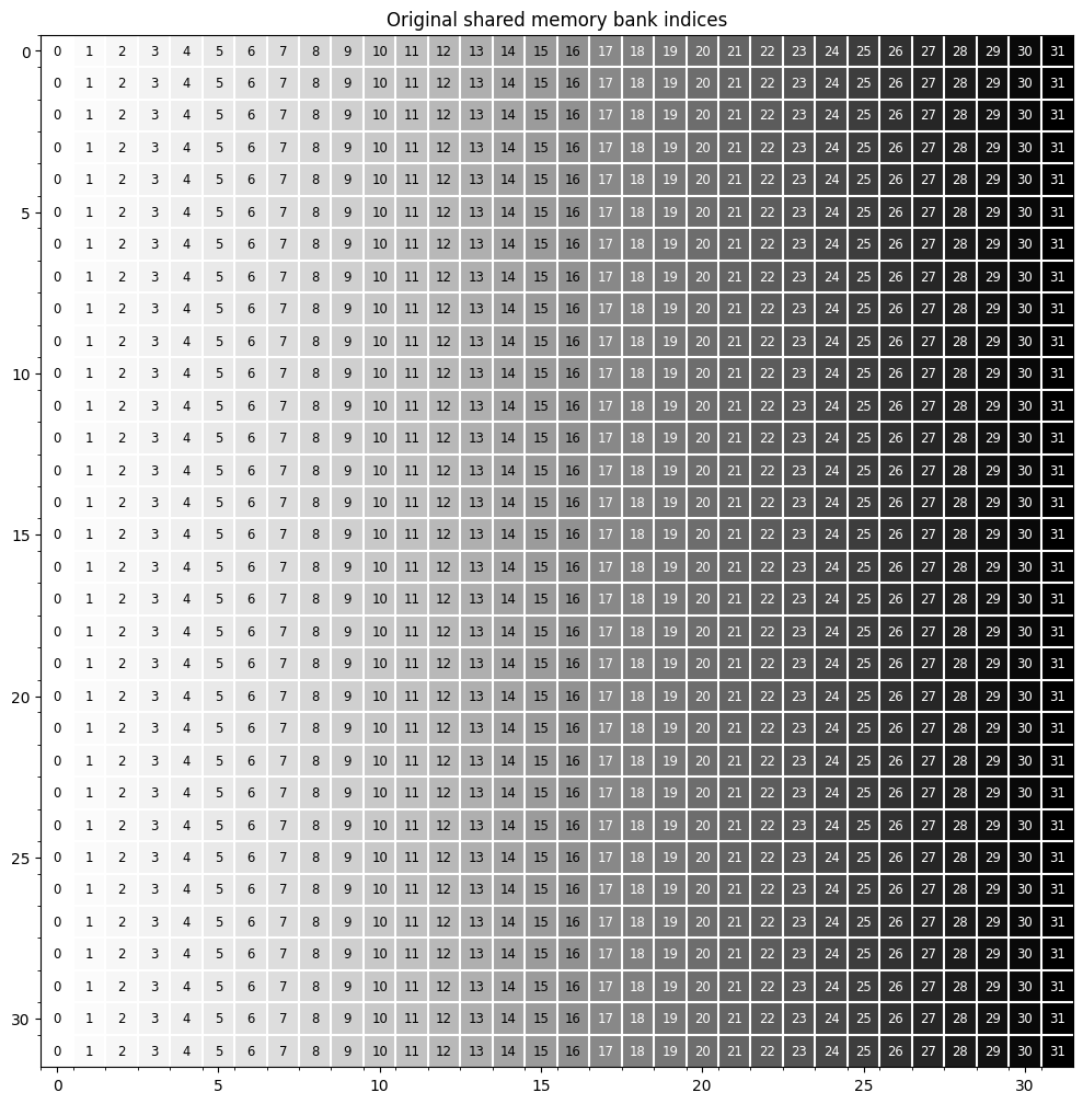
Swizzle toy example: original bank indices

A toy example: the indices of the shared memory bank each element is mapped to.

In a toy kernel, suppose each warp accesses an entire row of the matrix: for warp 0, thread 0 accesses the element at $[0, 0]$, thread 1 accesses $[1, 0]$, and so on. Because all of these accesses map to the same shared-memory bank, this results in a 32-way bank conflict. To avoid this, we apply a swizzle to the matrix layout.

In this case, there is no need to group elements together, so we set MBase = 0. Each row contains 32 elements spanning all 32 banks that need to be permuted while keeping the row index unchanged. That means we only need to permute the 5 least significant bits of the column index (since $2^5 =32$), so we set BBits = 5 and SShift $= log_{2}(32) - 0 = 5$.

Using Mbase = 0, BBits = 5, SShift = 5 parameters results in the following updated bank indices.

Swizzle toy example: updated bank indices

A toy example: the updated indices of the shared memory bank each element is mapped to.

All elements in each row is now mapped to different banks, which eliminates bank conflicts.

As data loads

For 2-byte elements, 64 elements span all 32 shared-memory banks. As part of the ldmatrix operation, a group of four consecutive threads collectively loads 16 bytes when reading an 8x8 matrix. This implies that eight 2-byte elements must remain contiguous. As a result, the 64 elements are organized into $64 / 8 = 8$ groups to be permuted.

Accordingly, we set MBase $= log_{2}(8) = 3$, BBits $=log_{2}(8) = 3$, and SShift $= log_{2}(64) - $ Mbase $= 3$.

When only a single 8x8 matrix is loaded, the swizzle is sufficient to eliminate bank conflicts. However, as the number of 8x8 matrices loaded per instruction increases, bank conflicts become unavoidable because the additional elements must reuse the same banks. Specifically, using .num = .x2 results in 2-way bank conflicts with the swizzle applied (which is an improvement over the 4-way bank conflicts observed without swizzling; see the figure below). With .num = .x4, bank conflicts rise to 4-way, matching the conflict level observed without any swizzle.

Original bank indices the elements of As are mapped to

The original bank indices the elements of As are mapped to where the four 8x8 matrices loaded by ldmatrix lead to 4-way bank conflicts.

Since swizzling does not reduce bank conflicts in this case, we do not apply it to As.

Bs data loads

In the current configuration, Bs has dimensions $16 \times 128$, which means that loading two 8x8 matrices vertically leads to 16-way bank conflicts. By applying the same swizzle parameters discussed in the As data loads section (MBase = 3, BBits = 3, and SShift = 3), we are able to reduce these conflicts to just 2-way bank conflicts.

Bank indices in Bs

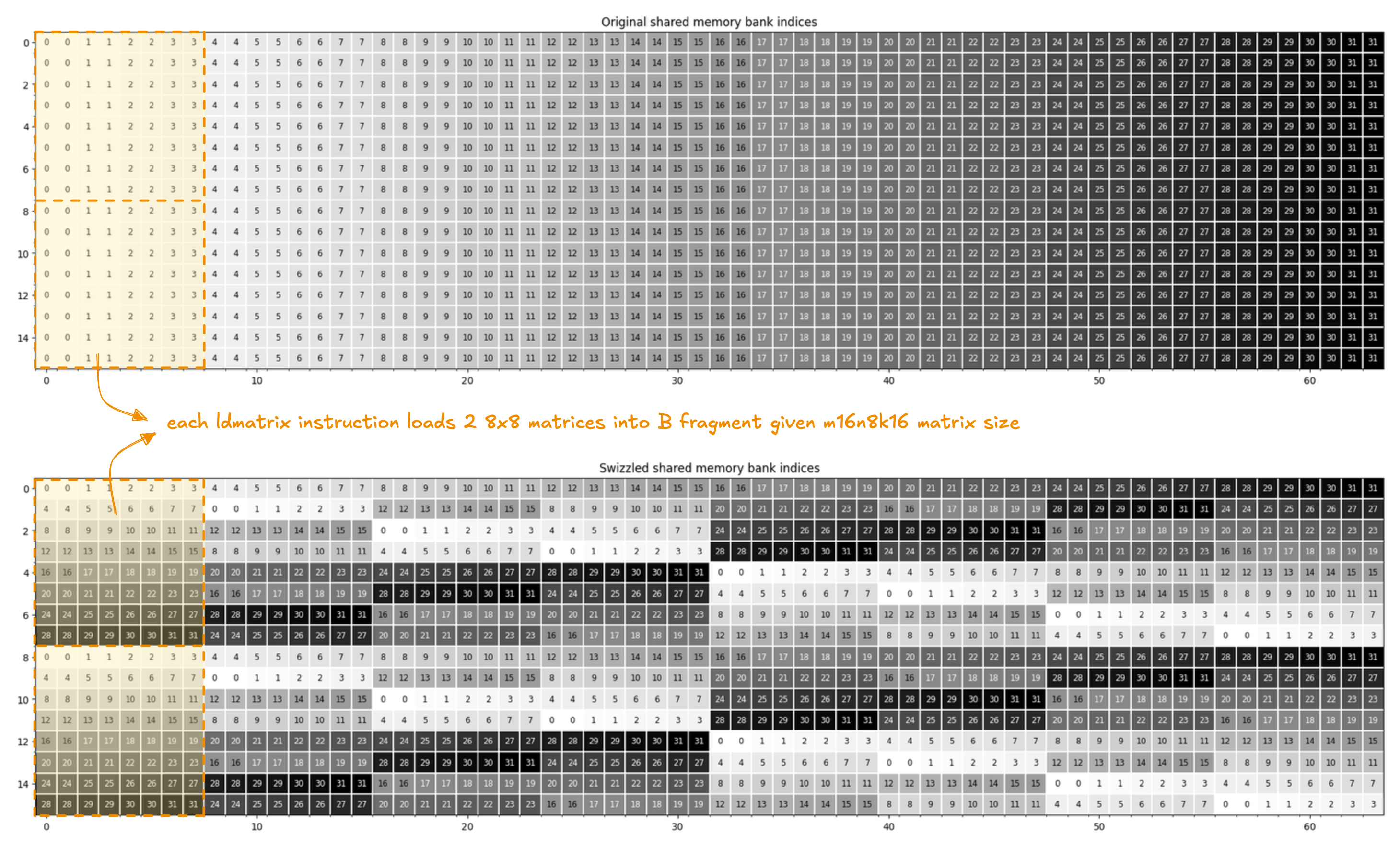
The original and the swizzled bank indices the elements in Bs are mapped to. The swizzle method reduces the bank conflicts from 16-way to 2-way.

The Python notebook that was used to produce the figures can be found here.

Summary

Applying the swizzle configuration to Bs boosts throughput to 84.24 TFLOPs/s, and incorporating the three-stage pipelining technique from Kernel 12 further increases it to 90.31 TFLOPs/s, exceeding 100% of cuBLAS performance!

Kernel #	Performance (TFLOPs/s)	% cuBLAS performance
cuBLAS	88.81	100%
kernel 06: warp tiling, subdivided	27.23	30.66%
kernel 09: tensor cores (wmma API)	65.38	73.62%
kernel 10: tensor cores + async gmem loads	73.77	83.06%
kernel 11: tensor cores + double buffering	80.33	90.45%
kernel 12: tensor cores + three-stage pipeline	87.13	98.11%
kernel 13: tensor cores (mma)	76.93	86.62%
kernel 14: tensor cores (mma) swizzled 🆕	84.24	94.85%
kernel 15: tensor cores (mma) swizzled + three-stage pipeline 🆕	90.31	101.69%

7. Summary

My original goal was simply to learn SGEMM optimization and implement a single Tensor Cores-based kernel, so I did not expect to end up exploring many additional techniques such as swizzling and pipelining. In my experience, wrapping my head around warp tiling (especially the subdivided variant), along with understanding how to use mma instructions and apply swizzling, required relatively more efforts. I’m glad I was able to work through and cover these topics. Again, if you notice any mistakes, issues, or have any feedback at all, I would love to hear it!

Note that I did not perform extensive parameter tuning. Instead, I experimented with a limited number of configurations and selected one that produced reasonably good performance for the chosen values of $M$, $N$, and $K$. The same configuration is unlikely to be optimal for other matrix shapes.

Overall, this post focuses on optimizing both SGEMM and MP-GEMM. For matrices of size $M = N = K = 4096$, we achieve beyond 95% of cuBLAS performance for SGEMM and beyond 101% of cuBLAS performance for MP-GEMM.

Resources

Matrix multiplication optimization posts

How to Optimize a CUDA Matmul Kernel for cuBLAS-like Performance: a Worklog by Simon Boehm (2022).
How To Write A Fast Matrix Multiplication From Scratch With Tensor Cores by Alex Armbruster (2024).

Optimization concepts and techniques

Understanding the Roofline Model taken from MIT 6.S894: Accelerated Computing Resources page
Asynchronous Data Copies section, Advanced Performance Optimization in CUDA by Igor Terentyev (2024).
Cute Swizzle implementation code.
CuTe Swizzle by Lei Mao (2024).
NVIDIA Tensor Core Programming by Lei Mao (2023).
HGEMM example code: Toy-HGEMM by DefTruth.

Documentation

Others

A significant number of questions and answers on the NVIDIA developer forums, where the majority were contributed by Robert Crovella.
Illustrations were drawn with Excalidraw.
Godbolt was used for sharing and viewing PTX instructions.

1. What does GEMM do?

2. Compute-bound or memory-bound? Introducing the roofline model

Example: determining whether the naive implementation is memory- or compute-bound

3. Problem setup

4. Single-precision GEMM implementations

🚨 CAUTION 🚨

Kernel 01: Naive implementation

If You're Curious...

Author's Note

Kernel 02: Block tiling

Author's Note

Author's Note

Kernel 02 in the Roofline Model

Kernel 03: 2D thread coarsening

Kernel 04: Vectorized memory access

Kernel 05: Warp tiling

Author's Note

Kernel 06: Warp tiling, subdivided

Author's Note

Kernel 07: Transposing As

Author's Note

Kernel 08: Asynchronous global-memory loads + double buffering

5. Tensor Cores

Author's Note

6. Mixed-precision GEMM implementations

If You're Curious...

Kernel 09: Tensor Cores (wmma API)

Author's Note

If You're Curious...

Author's Note

Kernel 10 & 11: Tensor Cores + asynchronous gmem loads + double buffering

Kernel 12: Tensor Cores + three-stage pipeline

Kernel 13: Tensor Cores (mma instructions)

If You're Curious...

Author's Note

Kernel 14 & 15: Swizzled shared memory + three-stage pipeline

7. Summary

Resources

Kernel 07: Transposing `As`