Reduction (Sum): part 1 | Introduction
In this series, we will explore how to implement parallel sum reduction using CUDA. We’ll begin with an introductory post covering the following key topics:
- What is sum reduction, and how can we parallelize it?
- Choosing memory bandwidth as the metric
- Utilizing shared memory
- Setting up the implementation code
We’ll then dive into the implementation details and optimization techniques for reduction in Part 2.
Note: this post assumes that the readers are already familiar with threads and blocks in GPU programming. The Github link to the implementation code can be found here.
1. What is sum reduction, and how can we parallelize it?
Given a list of elements, reduction applies an operation on each of the elements and accumulates them into one single value, hence, the term “reduce”. In the case of sum reduction, the operation sums all the elements together, outputting the final sum value. For instance, with a list of length 8 containing the elements [1, 2, 3, 4, 5, 6, 7, 8], the sum reduction output would be 1 + 2 + 3 + 4 + 5 + 6 + 7 + 8 = 36. Other reduction operations include, but are not limited to, max, min, and mean.
To implement sum reduction, the most naive way is to add the elements sequentially:
int array[] = {1, 2, 3, 4, 5, 6, 7, 8};
int N       = 8;
int output  = 0; // For storing the sum reduction output; initialize to 0.

for (size_t i{0}; i < N; ++i) {
    output += array[i];
}
The above solution requires 8 time steps to complete, and this O(N) approach does not scale well with large inputs. So to improve performance and better utilize available resources (e.g., the GPU), we can restructure it as a tree-based approach:
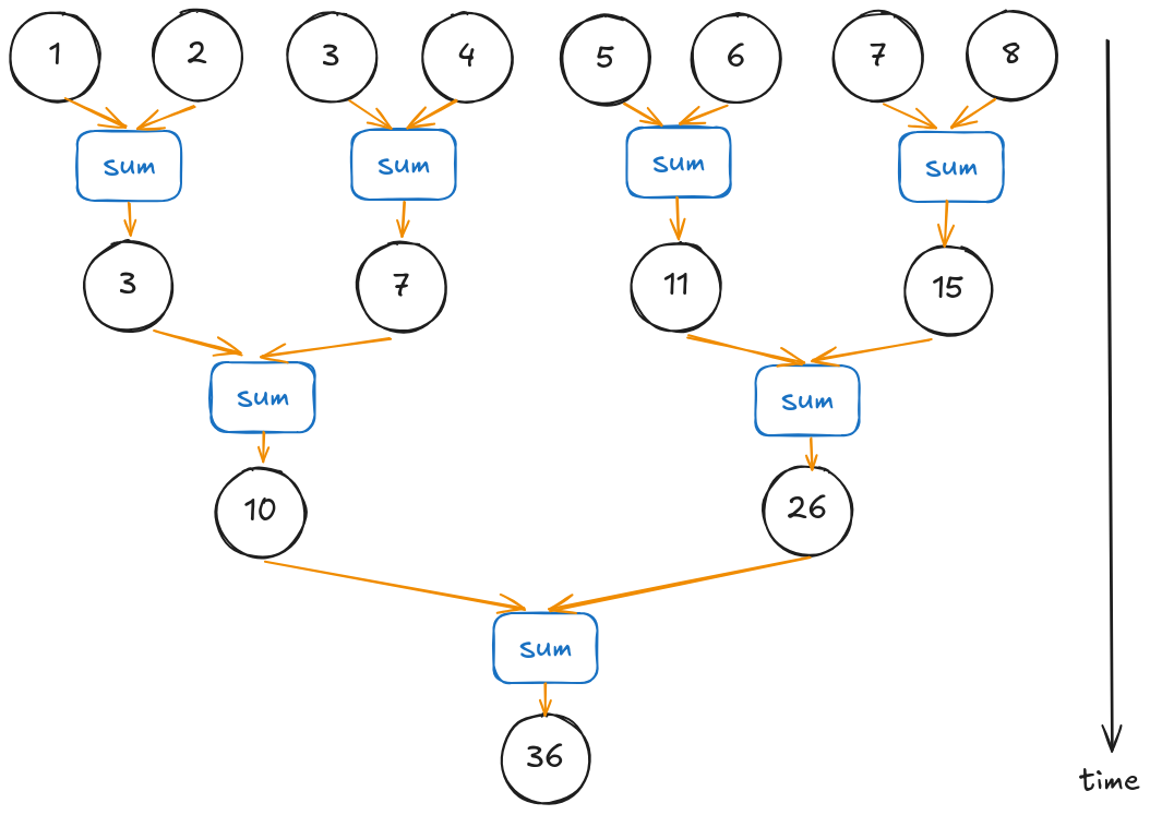
One tree-based approach to parallelize our problem example.
Compared to the 8 time steps in the sequential approach, it now only requires 3 time steps: 4 sum operations in the first step, 2 sum operations in the second step, and one final sum operation in the third step.
Note that here, we assume sufficient resources to perform all 4 sum operations simultaneously. In practice, however, often the data is so large that we need to break the computations into multiple batches, with each batch handled by a separate thread block. Once we obtain the partial sum from each batch, we then invoke the reduction kernel one more time with a single block to compute the final sum.
The figure below illustrates this process: the kernel is first launched with 8 blocks to compute 8 partial sums from the input elements. These partial sums are then passed to a second kernel launch, now using a single block, to produce the final result.
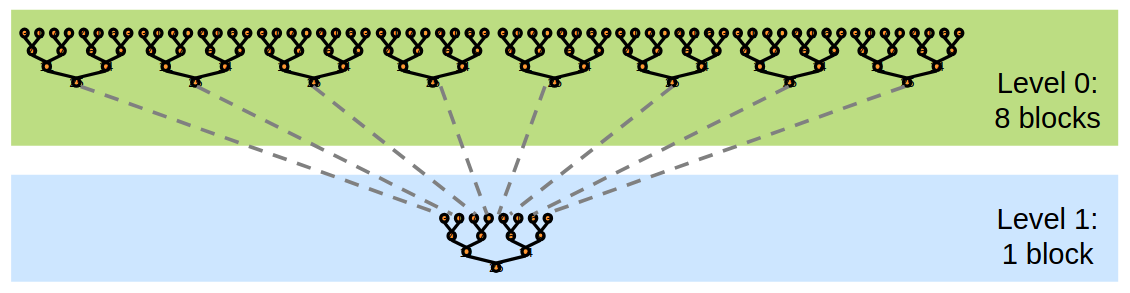
We may need to perform multiple kernel invocations to handle large datasets. Figure taken from Mark Harris's deck.
2. Choosing memory bandwidth as the metric
Reduction is an example of memory-bound kernels: for each element loaded, only one floating-point operation is performed. In such cases, optimizing memory access efficiency becomes the priority where we strive to reach the GPU peak bandwidth. In contrast, compute-bound kernels, such as matrix multiplication, are limited by arithmetic intensity rather than memory access. We will look into matrix multiplication in a future post.
What is my GPU peak memory bandwidth?
There are two ways to obtain the GPU peak memory bandwidth. One is to look up the specifications. For example, I’m using the RTX 5070 Ti, and according to the specification document, the memory bandwidth is 896 GB/s.
Another way is to calculate the peak bandwidth by multiplying the memory bus width and memory clock speed obtained from cudaGetDeviceProperties:
// Code taken and slightly modified from Lei Mao's reduction article: https://leimao.github.io/blog/CUDA-Reduction/.
int device_id{0};
cudaGetDevice(&device_id);
cudaDeviceProp device_prop; // For storing the device properties.
cudaGetDeviceProperties(&device_prop, device_id);

// Calculate peak bandwidth:
// 1) Obtain memory clock rate in kHz and convert to Hz.
// Note that memoryClockRate is deprecated in CUDA 12.x and removed in CUDA 13.
double const memory_clock_hz{device_prop.memoryClockRate * 1000.0};

// 2) Obtain memory bus width in bits and convert to bytes.
double const memory_bus_width_bytes{device_prop.memoryBusWidth / 8.0};

// 3) Factor of 2.0 for Double Data Rate (DDR), then divide by 1.0e9 to convert from bytes/s to GB/s.
// The result (for RTX 5070 Ti) should roughly be 896 GB/s.
float const peak_bandwidth{static_cast<float>(2.0f * memory_clock_hz * memory_bus_width_bytes / 1.0e9)};
Memory clock rate determines the rate to which data is transferred to and from the GPU in kHz. Memory bus width determines the number of bits that can be simultaneously transferred to and from the GPU. We then incorporate Double Data Rate (DDR), where data is transferred twice per clock cycle since it’s transferred on both rising and falling edges of the clock signal.
In brief, we aim to reach for the GPU peak memory bandwidth (896 GB/s on RTX 5070 Ti) in our optimization efforts.
3. Utilizing shared memory
In section 1, we have discussed how we can restructure the sequential sum reduction into a tree-based approach. Suppose each sum operation in one time step is performed by a single thread. How can we enable the threads in the next time step to access the outputs of the sum operations computed in the previous time step?
One naive approach is to store the intermediate outputs in global memory. For instance, we can allocate an array in global memory and initialize it with the input values. At each time step, every thread loads two relevant values from the array, computes their sum, and writes the result back to the array. Synchronization is required to ensure that all threads have completed their operations at each time step before the next begins.
However, accessing global memory is slow, so having to access it so many times in the kernel would surely affect the performance significantly. This is where shared memory comes in.
Shared memory resides on-chip, giving it significantly higher throughput compared to global memory, which is located in the GPU’s off-chip DRAM. Shared memory is allocated per thread blocks, which means that all threads within a block can access the same shared memory variables. However, it has a much lower capacity compared to global memory; depending on how much shared memory each block requires, it may limit the number of blocks that can be placed on each Streaming Multiprocessor (SM). You can read more about shared memory here.
Author's Note
"How CUDA Programming Works" presentation by Stephen Jones provides a really good explanation of how the resources required by each thread block, such as shared memory, affect the number of blocks that can be scheduled on each SM. The slide below, taken from the presentation, illustrates an example of this.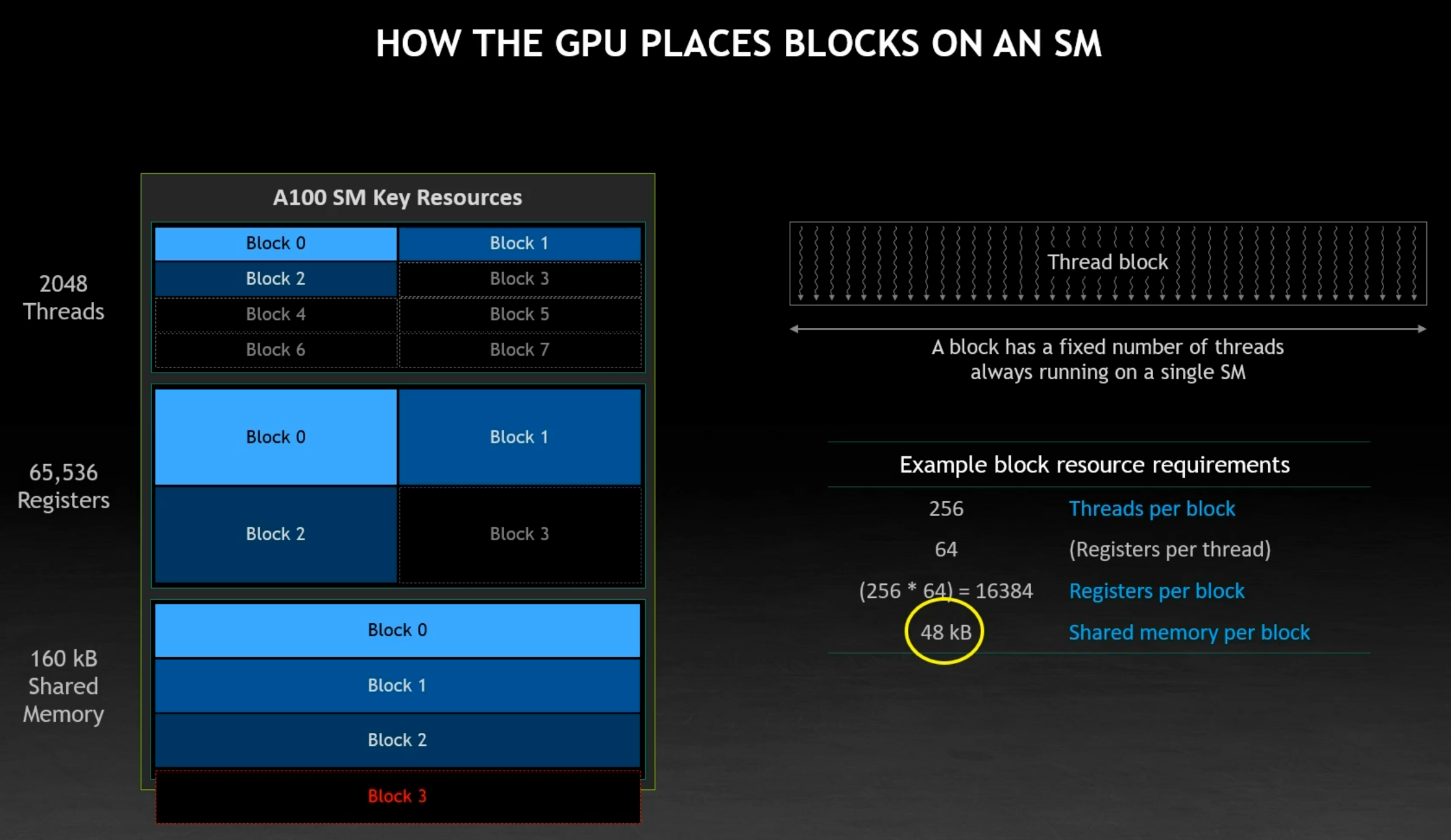
Given the block resource requirements (shown in the table on the right), we can see that the GPU is unable to place Block 3 due to the insufficient remaining shared memory. Since 3 blocks have already been placed ($3 \times 48\ kB = 144\ kB$), only $160\ kB - 144\ kB = 16\ kB$ of shared memory capacity remains, which is insufficient for another block that requires 48 kB.
We will use shared memory in all of the sum reduction implementations discussed in Part 2. For example, the first few implementations require # threads per block * sizeof(float) bytes of shared memory per thread block, so that each thread has its own slot.
4. Setting up the implementation code
I used and slightly modified Lei Mao’s reduction code setting as follows.
- Error handling, output verification, and performance measurement: I include error handling (
CHECK_CUDA_ERROR()andCHECK_LAST_CUDA_ERROR()), kernel output verification (withinprofile_batched_kernel()), and performance measurement (measure_performance_in_ms), with minor variable/function renaming based on personal preferences. They can be found inutils.cuh. - Cache flush kernel: To ensure accurate benchmarking when running the reduction kernels on smaller datasets, I included a cache-flush kernel. This prevents inflated effective memory bandwidth caused by repeated runs benefiting from cached data.
- Improved memory management: instead of allocating, freeing, and reallocating device memory for each kernel invocation, I now allocate and free memory once in
main()(seerun_kernel.cu). This reduces overhead and speeds up the overall process without affecting the kernel performance. - Kernel organization: all kernel implementations are located in the
kernelsdirectory. This organization was inspired by Simon’s matmul kernel optimization repo.
Computing the effective bandwidth
Recall in section 1 that we may need to perform multiple kernel invocations to obtain the final sum. In this post, we primarily want to measure the effective memory bandwidth of only the first kernel invocation to align with both Lei Mao’s and Mark Harris’s implementations. This means that we would 1) load all the elements from the input list from the global memory and 2) store the partial sums of each batch at the end of the kernel execution back to the global memory.
The calculation for getting the effective memory bandwidth can be found below.
// Assume num_elements and batch_size have been defined (see additional notes).
// Assume latency has been computed (see additional notes).

// Total bytes transferred = bytes loaded (i.e., all the elements from the input list) +
//                           bytes stored (i.e., number of batches/thread blocks, when partial sums are stored).
size_t num_bytes{num_elements * sizeof(float) + batch_size * sizeof(float)};

// Compute effective bandwidth in GB/s.
float const effective_bandwidth{(num_bytes * 1e-6f) / latency};
Additional notes
num_elements denotes the total number of elements in our input list, while batch_size specifies the number of thread blocks.
latency is measured using the following steps:
- Warmup the kernel. Run the kernel at least once to clear out any initial overheads and bring the system to a steady, optimal state. The warmup run is typically slower, so we don’t include it in the final measurement.
- Execute the kernel multiple times. This helps smooth out variability in runtime and provides more consistent results.
- Compute the average latency. Averaging the runtimes over several runs leads to more reliable estimate than measuring a single execution.
The steps above can be found in measure_performance_in_ms() function.
Problem setup
We have a list of 229 = 536,870,912 floating-point elements. The length itself was chosen arbitrarily, as long as it’s large enough and is also divisible by 1024.
🚨 CAUTION 🚨
Since the length is divisible by 1024, we don't include any boundary check in any of the kernel implementations for simplicity. In real-world applications, however, boundary checks are essential to prevent out-of-bounds memory access, which can lead to undefined behavior or crashes.The elements in Lei Mao’s post are all set to a constant value 1.0f. It significantly speeds up verification as the expected partial sum for each batch is simply the number of elements in the batch multiplied by the constant. However, I found that this problem setup is prone to a specific bug: incorrect shifting of the input list when running the kernel, which can go unnotized because all elements are identical. To address this, I created two subclasses of Elements, each differing in how they initialize values and perform verification:
-
RandomElements: initializes each element with a random floating-point value. During the verification, the partial sum of each batch is compared against the CPU-computed sum. This approach provides better test coverage but may be slower due to the large input size. -
ConstantElements: reproduces the setup from Lei Mao’s post. Each element is initialized to a constant value provided to the constructor. Verification is faster but more prone to undetected bugs due to uniformity in data.
When implementing the kernels, I first used RandomElements to verify that the code produced correct results. I then switched to ConstantElements for benchmarking purposes.
The definition of all element classes can be found in elements.h file.
With the basics covered, we are now ready to implement and optimize the sum reduction algorithm! Click here to continue to the next part of the series.
Resources
- Optimizing Parallel Reduction in CUDA by Mark Harris (2007)
- CUDA Reduction by Lei Mao (2024)
- Using Shared Memory in CUDA C/C++ by Mark Harris (2013)
- Illustrations were made with Excalidraw