Reduction (Sum): part 2
As part of the “Reduction (Sum)” series, this post outlines my process and approach to implementing and optimizing sum reduction kernels. I use Mark Harris’s Optimizing Parallel Reduction in CUDA deck and Lei Mao’s CUDA Reduction code as references, with modifications based on the insights I’ve gained along the way. My approach can be summarized as follows.
- Implement the reduction kernel and ensure that the output is correct using the verification process described in the previous post.
- Analyze the kernel’s performance to understand whether (and why) it performs better or worse. Some methods include:
- Profile the kernel using NVIDIA Nsight Compute. I highly recommend you to watch this kernel profiling lecture hosted by GPU Mode if you are interested in using Nsight Compute.
- Inspect the PTX/SASS, if necessary, to better understand the performance characteristics or identify optimization opportunities. I use Godbolt for convenient viewing and easy sharing.
Note that in this post, the terms batch and block are used interchangeably and will be treated as identical.
Kernel 0: naive interleaved addressing
This kernel follows closely the tree-based approach illustrated in the previous post. The implementation is summarized in the illustration below.
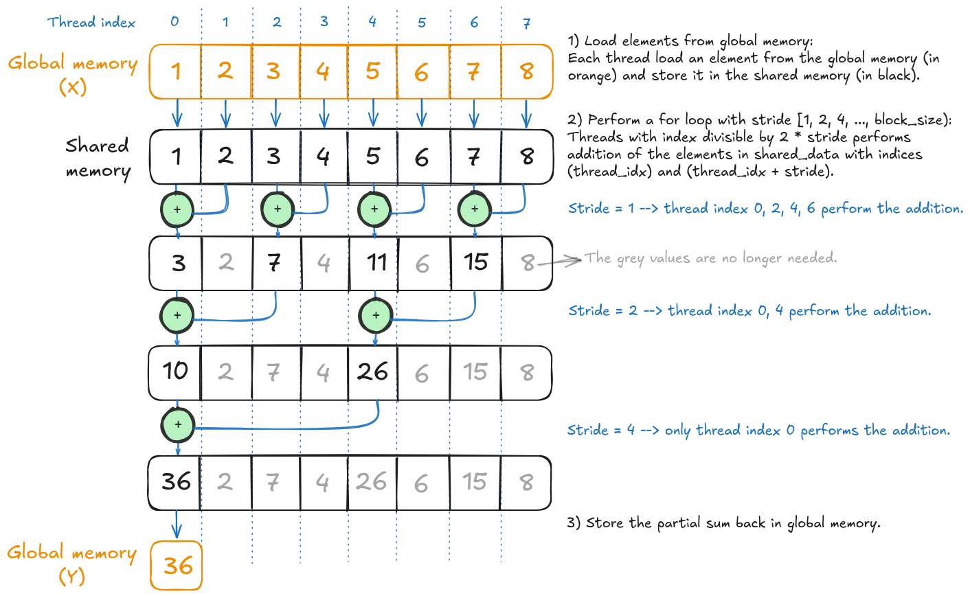
The first interleaved addressing kernel from Mark Harris's presentation.
The kernel function can be written as follows.
template <size_t NUM_THREADS>
__global__ void batched_interleaved_address_naive(
    float* __restrict__ Y,
    float const* __restrict__ X,
    size_t num_elements_per_batch
) {
    size_t const block_idx{blockIdx.x};
    size_t const thread_idx{threadIdx.x};
    // Allocate the shared memory with length of the number of threads in the block/batch.
    __shared__ float shared_data[NUM_THREADS];

    // Shift the input accordingly to the batch index.
    X += block_idx * num_elements_per_batch;
    // Store a single element per thread in shared memory.
    shared_data[thread_idx] = X[thread_idx];
    __syncthreads();

    for (size_t stride = 1; stride < NUM_THREADS; stride *= 2) {
        if (thread_idx % (2 * stride) == 0)
            shared_data[thread_idx] += shared_data[thread_idx + stride];
        __syncthreads();
    }

    if (thread_idx == 0)
        Y[block_idx] = shared_data[0];
}
Recall from the previous post that my GPU (RTX 5070 Ti) peak bandwidth is 896 GB/s and there are 229 number of elements. Running the kernel 50 times repeatedly with different numbers of threads per block leads to the following performance table.
| # Threads/block | Mean Effective Bandwidth | % Peak Bandwidth |
|---|---|---|
| 128 | 431.03 | 48.10 |
| 256 | 422.58 | 47.16 |
| 512 | 381.34 | 42.56 |
| 1,024 | 212.07 | 23.67 |
We observe that using 128 threads yields the best performance among all the options. Increasing the number of threads to 256 slightly degrades performance. Using 512 threads reduces it further, and with 1,024 threads, performance drops significantly where the achieved bandwidth is approximately half that of the 128-thread configuration.
What explains the performance differences across thread configurations?
Let’s start with the 1,024-thread configuration. The previous post briefly touched upon how the resources required by each block can limit the number of blocks that can be scheduled in each multiprocessor. These resources include the number of threads, the number of registers, and the amount of shared memory required per block.
The maximum threads per multiprocessor on my GPU is 1,536 (equivalent to 48 warps), as reported by the maxThreadsPerMultiProcessor field from cudaGetDeviceProperties. With a block size of 1,024, the GPU can only place 1 block (i.e., 32 warps) per SM. This means that out of the 48 warps slots available on the SM, only 32 are active, resulting in a theoretical occupancy of $32 / 48 \times 100\% = 66.67\%$. In contrast, the other thread configurations are able to achieve 100% theoretical occupancy.
As mentioned earlier, the number of registers and the amount of shared memory per block can also limit occupancy. However, this is not the case for any of the thread configurations used here for this particular kernel.
What about the remaining thread configurations? Why does the 128-thread configuration perform the best?
Looking at the profile generated by Nsight Compute, all three thread configurations exhibit thread divergence.

One of the suggested improvement opportunities from Nsight Compute, which is to address the thread divergence issue.
In our case, thread divergence occurs because the threads performing the sum operation in the for loop (i.e., the active threads whose indices satisfy the if condition) are scattered across multiple warps. In the 128-thread configuration, there are 64 active threads during the first iteration, but these threads are not grouped contiguously. The active threads consist of those with indices 0, 2, 4, 6, and so on. As a result, all 4 warps are partially active and must execute the loop body, leading to warp divergence. In ideal scenario, only 2 warps would be fully active and the remaining warps inactive, minimizing divergence.
Larger thread blocks can be more negatively affected by thread divergence since more warps increase the opportunity for divergence, which may help explain why the runtime worsens as the number of threads per block increases from 128 to 256 and 512.
We will only use the 128-thread configuration for all the subsequent implementations.
Kernel 1: interleaved addressing with thread divergence resolved
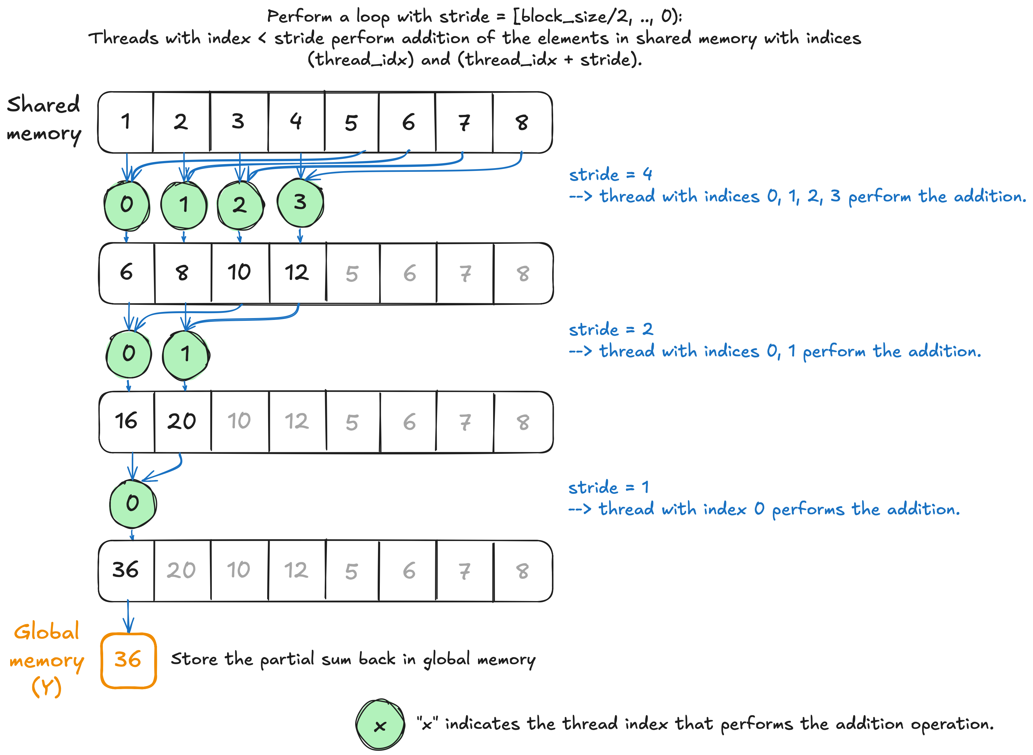
The only difference between Kernel 0 and Kernel 1 lies in how we select the active threads, i.e., the threads that perform the sum operation. The goal is to ensure that the active threads are contiguous such that only ceil(# active threads / 32) warp(s) are active. The figure below summarizes the implementation, with the global memory loading step omitted for brevity.
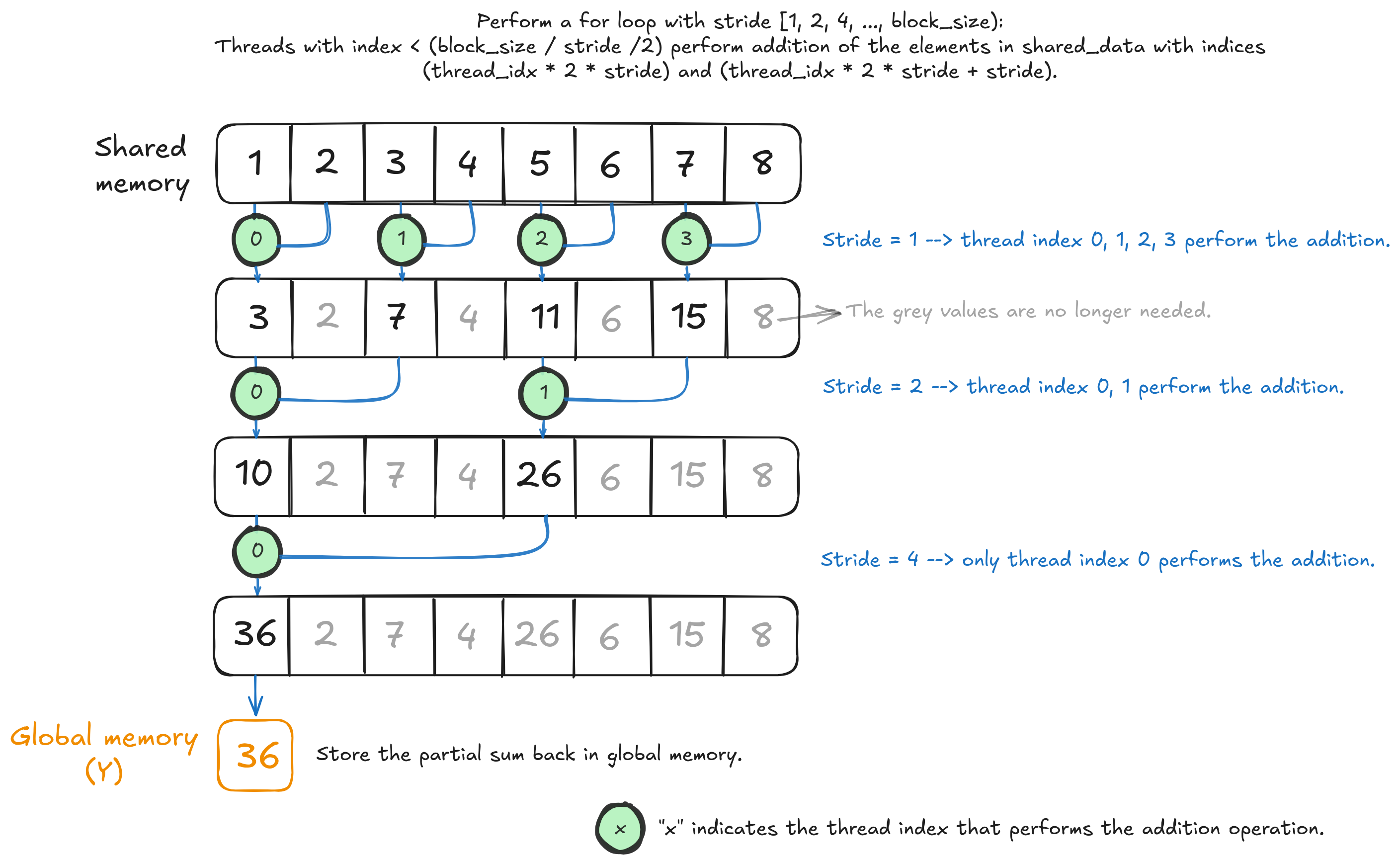
The interleaved addressing kernel with thread divergence resolved.
As for the code, we only need to change the following:
    for (size_t stride = 1; stride < NUM_THREADS; stride *= 2) {
        if (thread_idx % (2 * stride) == 0)
            shared_data[thread_idx] += shared_data[thread_idx + stride];
        __syncthreads();
to:
    for (size_t stride = 1; stride < NUM_THREADS; stride *= 2) {
        size_t index = 2 * stride * thread_idx;

        if (index < NUM_THREADS)
            shared_data[index] += shared_data[index + stride];
        __syncthreads();
    }
Below is the updated performance table.
| Kernel # (128 threads/block) |
Mean Effective Bandwidth | % Peak Bandwidth |
|---|---|---|
| kernel 0 | 431.03 | 48.10 |
| 🆕 kernel 1 🆕 | 434.87 | 48.53 |
There is a tiny improvement from Kernel 0 to Kernel 1, although it’s not particularly significant.
When profiling the kernel with Nsight Compute, we identify a new performance optimization opportunity: addressing Shared Load Bank Conflicts.

A new optimization opportunity observed on Nsight Compute: addressing bank conflicts.
What are shared memory bank conflicts, and why does Kernel 1 have this issue?
To answer this question, we need to examine how shared memory is organized. According to CUDA C++ Programming Guide, for devices with compute capability 12.0 (such as the RTX 5070 Ti), shared memory is divided into 32 banks or memory modules. This organization allows simultaneous access to n distinct addresses as long as they map to n different memory banks. Successive 32-bit words are mapped to successive banks, and each bank provides a bandwidth of 32 bits per clock cycle. A shared memory block containing 128 4-byte floating-point elements is organized as illustrated by the figure below.
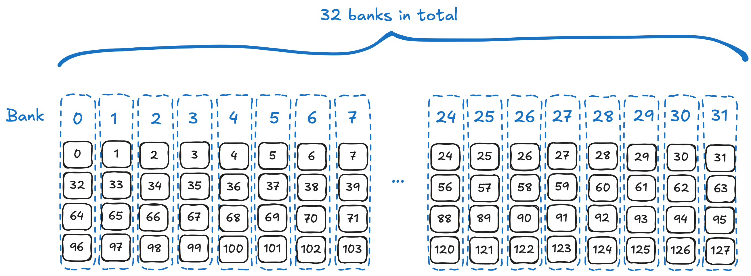
How the 128 elements are divided into 32 banks in the shared memory.
One or more bank conflicts occur when multiple threads in the same warp request different memory addresses that are mapped to the same memory bank. These accesses are then serialized, which consequently reduces the effective bandwidth by a factor equal to the number of the memory requests targeting that bank.
In Kernel 0, no bank conflicts occur because threads within the same warp always request addresses that are mapped to different banks. The figure below illustrates the read memory requests by threads in warp 0 (thread index 0 to 31) during the first two iterations of the for loop. In iteration 0 (stride = 1), thread 0 requests shared memory elements at indices 0 and 1 (located in bank 0 and 1, respectively), thread index 2 requests elements at index 2 and 3 (located in bank 2 and 3), and so on. The same pattern remains consistent across subsequent iterations and for all other warps.
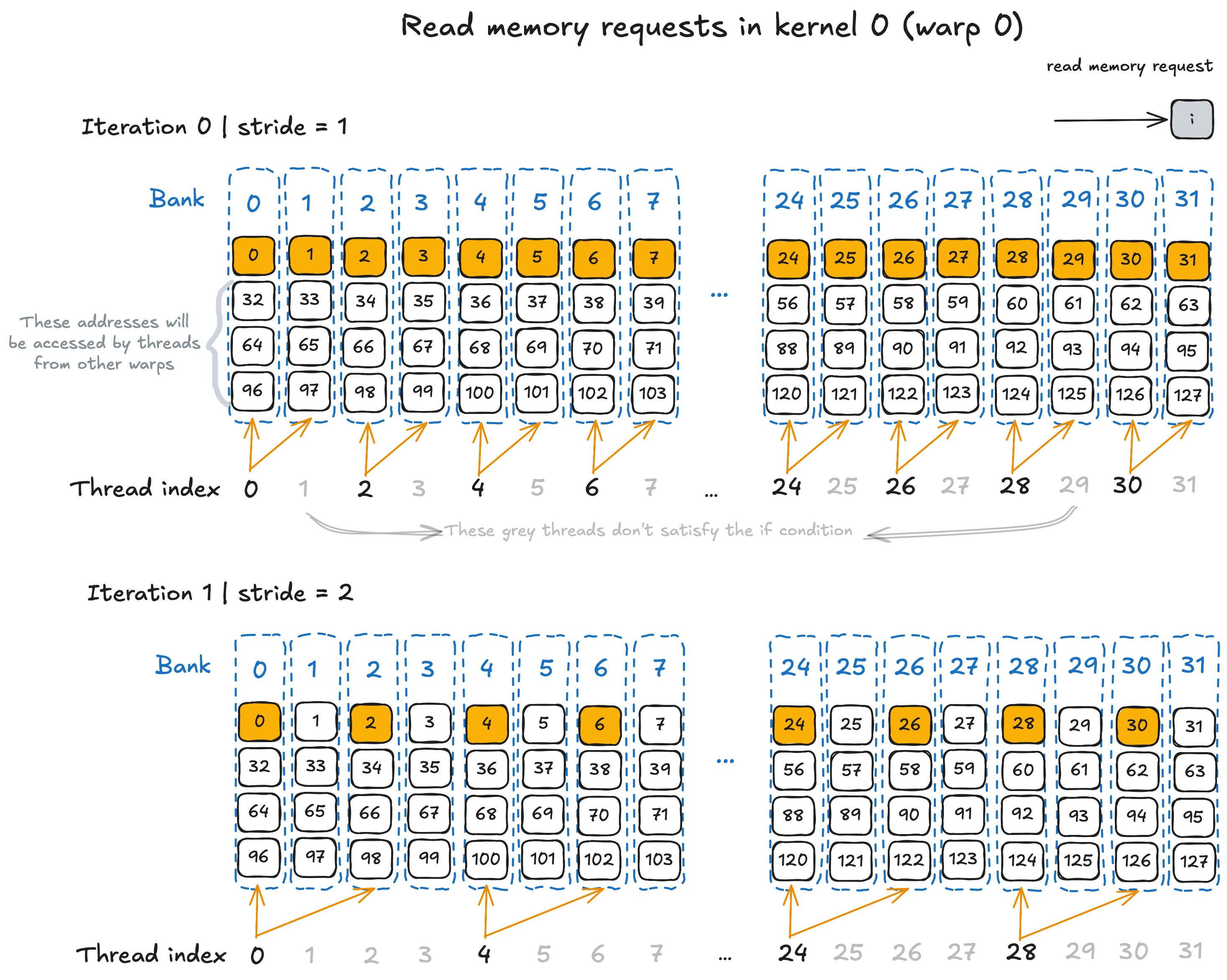
The memory requests by warp 0 threads in Kernel 0 during the first two iterations
In contrast, since the threads performing memory access are grouped into a contiguous block in Kernel 1, bank conflicts occur consistently in all iterations. The figure below illustrates the read memory accesses during the first two iterations, where a 2-way bank conflicts occur in the first iteration and 4-way bank conflicts occur in the second iteration. This behavior can significantly reduce the overall effective bandwidth.
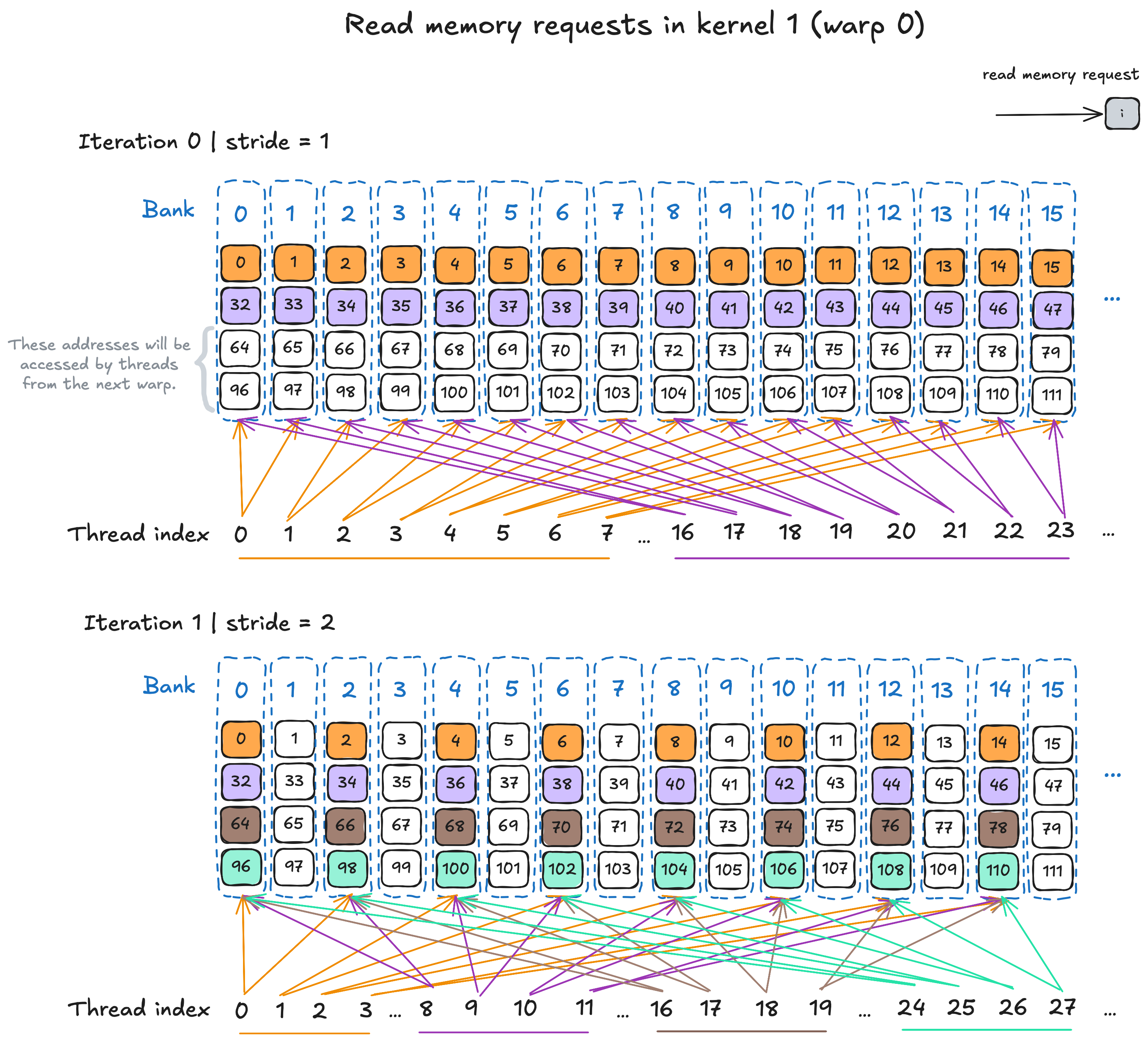
The memory requests by warp 0 threads in Kernel 1 during the first two iterations. Bank conflicts occur in both iterations.
In summary, although Kernel 1 resolves the thread divergence issue present in Kernel 0, the shared memory bank conflict issue still needs to be addressed.
Kernel 2: sequential addressing
The next implementation addresses the shared memory bank conflict issue observed in Kernel 1 by storing the intermediate sum values in sequential shared memory addresses. The following figure illustrates the updated approach.
The sequential addressing kernel.
In the code, we simply change the following rows from Kernel 1:
    for (size_t stride = 1; stride < NUM_THREADS; stride *= 2) {
        size_t index = 2 * stride * thread_idx;

        if (index < NUM_THREADS)
            shared_data[index] += shared_data[index + stride];
        __syncthreads();
    }
to:
    for (size_t stride = NUM_THREADS / 2; stride > 0; stride >>= 1) {
        if (thread_idx < stride)
            shared_data[thread_idx] += shared_data[thread_idx + stride];
        __syncthreads();
    }
Interestingly, we don’t observe any speedup between Kernel 1 and Kernel 2, which contrasts with nearly 2x performance improvement reported in Mark Harris’s presentation.
| Kernel # (128 threads/block) |
Mean Effective Bandwidth | % Peak Bandwidth |
|---|---|---|
| kernel 0 | 431.03 | 48.10 |
| kernel 1 | 434.87 | 48.53 |
| 🆕 kernel 2 🆕 | 434.73 | 48.51 |
What accounts for the discrepancy between the performance differences observed in this post and those reported in Mark Harris’s presentation?
One possible explanation is the improved shared memory performance under bank conflict conditions in newer GPU generations. While I haven’t been able to find any explicit statement from NVIDIA confirming this, a 2016 paper titled “Dissecting GPU Memory Hierarchy Through Microbenchmarking” demonstrated that newer GPU architectures at the time exhibited a lower performance penalty under bank conflict scenarios (see Table 8 in the paper). It’s worth noting that Mark Harris’s presentation dates back to 2007. It is possible that the penalty is even smaller on more recent architectures, such as Blackwell. That said, addressing shared memory bank conflicts remains important for achieving optimal performance.
Kernel 3: repositioning __syncthreads()
Kernel 2 includes two thread synchronizations: (1) after loading elements from global memory to shared memory, and 2) at the end of each for loop iteration to ensure all thread updates to shared memory are completed. We can further simplify this by removing one synchronization and repositioning the other to the beginning of the for loop.
By synchronizing threads at the start of the loop, we ensure that the initial shared memory load from global memory is complete before any computation begins. The only synchronization removed is the final one, which would have occurred at the end of the last iteration: when only a single thread updates the first shared memory element.
This removal is safe because the same thread that performs the final update is also responsible for writing the result back to global memory after the loop ends. Since no other threads are involved at this point, no synchronization is necessary.
To summarize, we change the following code:
    // Store a single element per thread in shared memory.
    shared_data[thread_idx] = X[thread_idx];
    __syncthreads(); // The first synchronization.

    for (size_t stride = NUM_THREADS / 2; stride > 0; stride >>= 1) {
        if (thread_idx < stride)
            shared_data[thread_idx] += shared_data[thread_idx + stride];
        __syncthreads(); // The second synchronization.
    }
to
    // Store a single element per thread in shared memory.
    shared_data[thread_idx] = X[thread_idx];

    for (size_t stride = NUM_THREADS / 2; stride > 0; stride >>= 1) {
        __syncthreads(); // The repositioned synchronization.
        if (thread_idx < stride)
            shared_data[thread_idx] += shared_data[thread_idx + stride];
    }
which gives us a better performance as shown below.
| Kernel # (128 threads/block) |
Mean Effective Bandwidth | % Peak Bandwidth |
|---|---|---|
| kernel 0 | 431.03 | 48.10 |
| kernel 1 | 434.87 | 48.53 |
| kernel 2 | 434.73 | 48.51 |
| 🆕 kernel 3 🆕 | 479.68 | 53.53 |
Kernel 4: thread coarsening
Recall in all the kernels so far, after loading elements from global memory into shared memory, half of the threads (N / 2) become idle at the start of the for loop. In the second iteration, N / 4 threads become idle, then N / 8 in the third, and so on, until only one thread remains active in the final iteration. This progressive underutilization of resources, exacerbated by the attempt to maximize parallelism (i.e., launching as many threads as possible), can significantly impact performance.
One fundamental optimization technique to address this issue is thread coarsening. The idea is to have each thread perform more work, thereby reducing the total number of threads launched and minimizing parallelization overhead. In this context, I’m merging Mark Harris’s Reduction #4 (First Add During Load) and Reduction #7 (Multiple Adds Per Thread), and will experiment with varying the number of elements each thread loads and adds. The implementation is illustrated by the figure below.
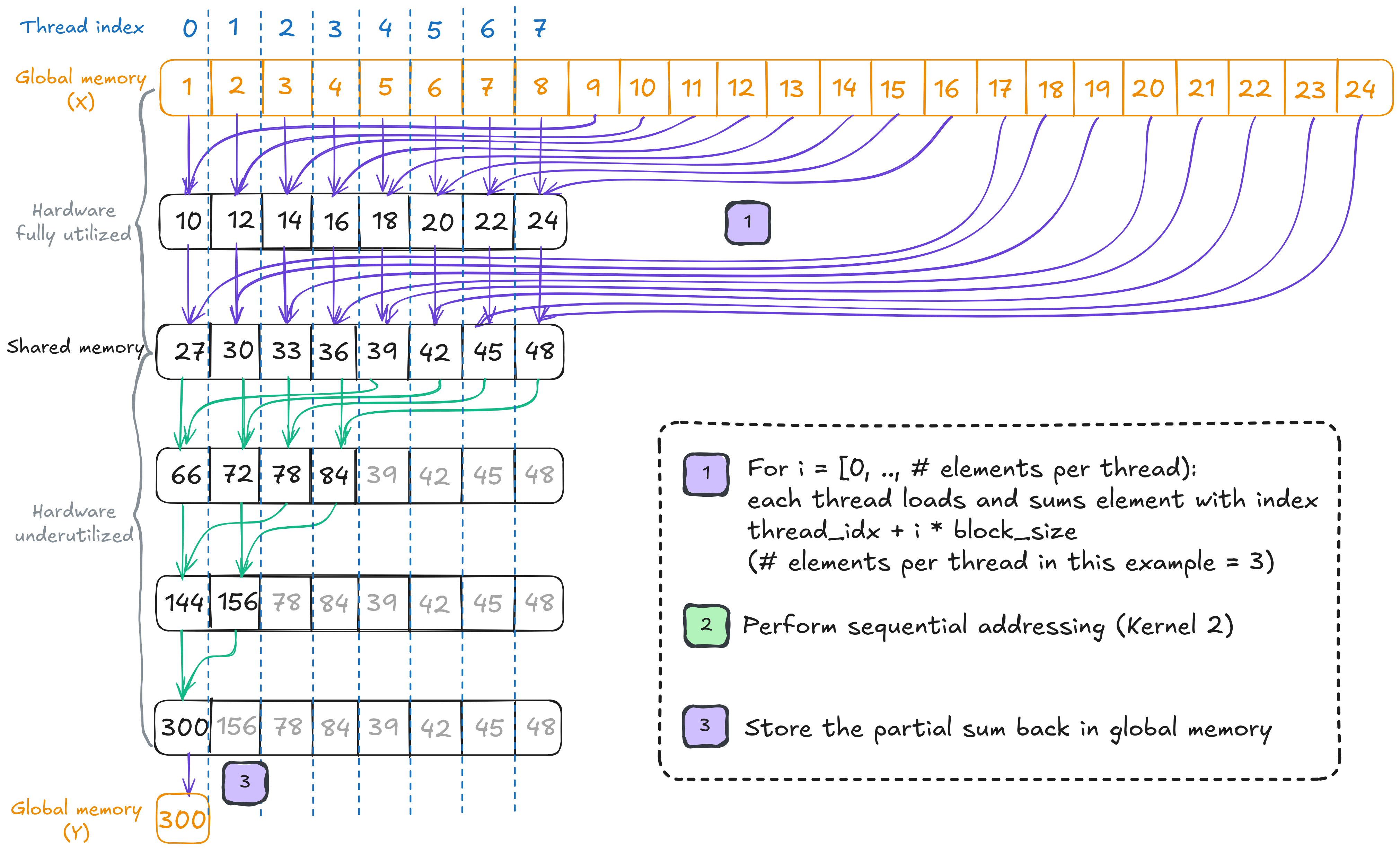
The thread coarsening kernel where the number of elements per thread is set to 3.
In the implementation code, we replace the code line that stores an element from global memory to shared memory:
    // Store a single element per thread in shared memory.
    shared_data[thread_idx] = X[thread_idx];
with the following for loop:
    // Compute the number of elements each thread will process.
    size_t const num_elements_per_thread{(num_elements_per_batch + NUM_THREADS - 1) / NUM_THREADS};

    // Initialize the sum variable.
    float sum{0.0f};

    for (size_t i = 0; i < num_elements_per_thread; ++i) {
        size_t const offset{thread_idx + i * NUM_THREADS};
        if (offset < num_elements_per_batch)
            sum += X[offset];
    }
    shared_data[thread_idx] = sum;
Experimenting with varying number of elements per thread using the 128-thread configuration leads to the following result.
| # elements per thread | Mean Effective Bandwidth | % Peak Bandwidth |
|---|---|---|
| 1 | 466.94 | 52.11 |
| 2 | 834.00 | 93.07 |
| 4 | 840.04 | 93.75 |
| 8 | 841.28 | 93.89 |
| 16 | 841.76 | 93.94 |
| 32 | 842.07 | 93.97 |
| 64 | 841.94 | 93.96 |
| 128 | 841.39 | 93.90 |
| 256 | 841.40 | 93.90 |
| 512 | 840.24 | 93.77 |
Based on the table above, we observe a significant performance jump: from 52% in the one-element-per-thread configuration to 93% in the two-elements-per-thread configuration! Performance continues to gradually improve as the number of elements per thread increases, peaking when each thread processes 32 or 64 elements.
Additionally, the Nsight Compute profiles show that achieved occupancy increases from 86% in Kernel 2 to 99% in Kernel 4 (recall that both kernels have a theoretical occupancy of 100%). This improvement is likely due to the significantly lower overhead associated with launching fewer threads and the overall better utilization of resources in Kernel 4.
Why are the elements being summed in each thread separated by a stride that is a multiple of the block size?
Notice that when computing offset in the for loop, each thread sums elements at indices of the form thread_idx + <multiple of NUM_THREADS>. You might wonder why we don’t simply sum n contiguous elements per thread, where n is the number of elements assigned to each thread.
As discussed in Part 1, global memory access is relatively slow, so optimizing memory access efficiency is critical. By introducing a stride (i.e., a gap between the elements each thread accesses), we ensure that all threads in a warp collectively access contiguous memory locations in each iteration (see the figure below). This pattern enables the hardware to potentially combine these accesses into a single memory transaction–a process known as memory coalescing, which significantly improves memory throughput.
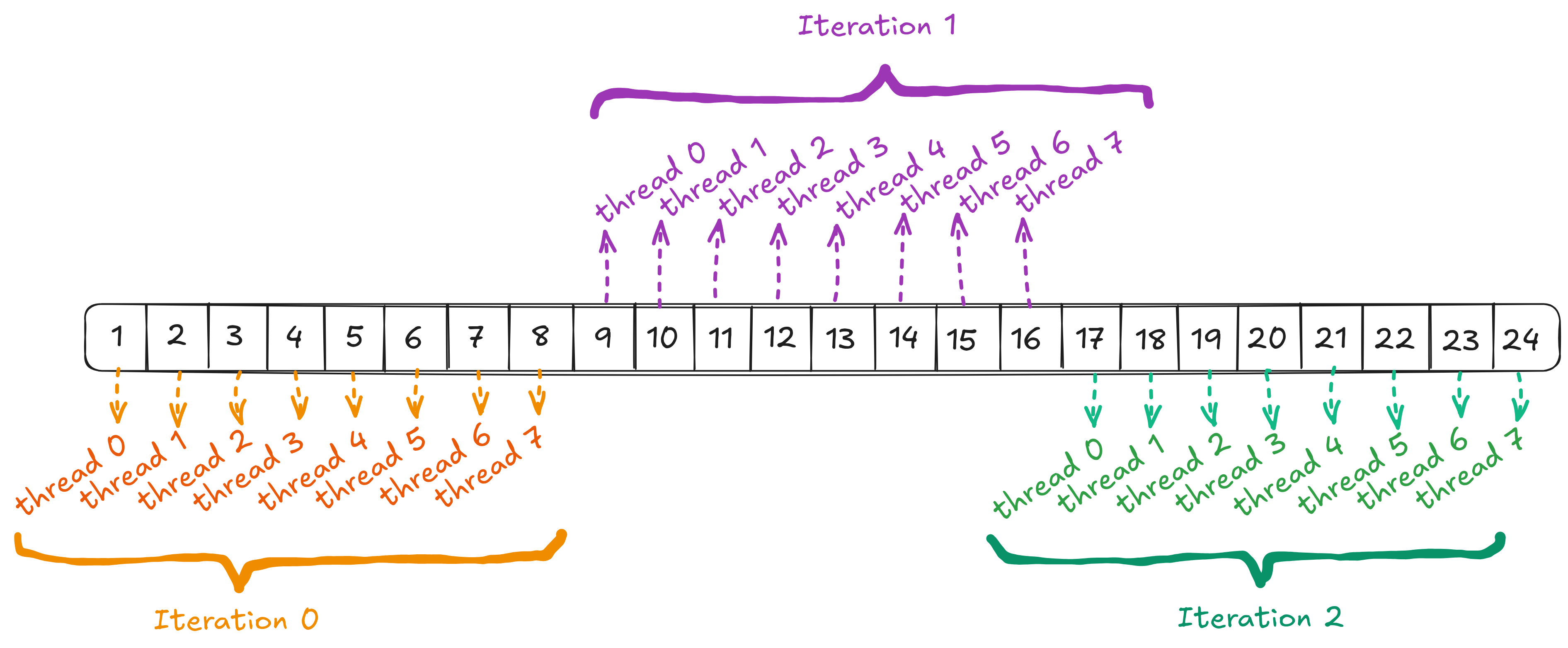
A coalesced access pattern in which contiguous memory locations are accessed during each for loop iteration.
If You're Curious...
Using an uncoalesced memory access pattern with 32 elements per thread results in an effective memory bandwidth of 769.54 GB/s, compared to 842.07 GB/s with coalesced access.To summarize, we have the updated performance table below.
| Kernel # (128 threads/block) |
Mean Effective Bandwidth | % Peak Bandwidth |
|---|---|---|
| kernel 0 | 431.03 | 48.10 |
| kernel 1 | 434.87 | 48.53 |
| kernel 2 | 434.73 | 48.51 |
| kernel 3 | 479.68 | 53.53 |
| 🆕 kernel 4 🆕 | 842.07 | 93.97 |
At this point, we have reached 94% peak bandwidth. Let’s see if the rest of the kernels in Mark Harris’s presentation can improve it even further.
Kernel 5: loop unrolling
Loop unrolling is an optimization technique in which developers or compilers rewrite a loop as a sequence of repeated, independent statements. The goal is to reduce or eliminate the overhead associated with loop control operations, such as index incrementation and end-of-loop condition checks. You can find more details here.
Mark Harris’s presentation provides two kernels that perform loop unrolling: Reduction #5 (Unroll The Last Warp) and Reduction #6 (Competely Unrolled).
🚨 CAUTION 🚨
The changes added to Reduction #5 is now obsolete on newer GPUs, which I will discuss further towards the end of the section. Feel free to skip to the next section.Reduction #5 (Kernel 5 v1): unroll the last warp
In this implementation, only the final active warp (i.e., threads with indices < 32) is unrolled. We do so by defining and calling a helper function warp_reduce where these threads perform the summation without requiring any explicit thread synchronization. This is possible because all threads within a warp in older GPUs execute in lockstep, meaning, all active threads follow the same instruction stream simultaneously, and none can advance ahead or fall behind. As mentioned, that this strict lockstep behavior applies primarily to older GPU architectures. We’ll discuss the implications of this later when addressing potential issues.
To implement the kernel, we add three modifications to the code:
1. Define the helper function warp_reduce().
__device__ void warp_reduce(volatile float* shared_data, size_t thread_idx) {
    shared_data[thread_idx] += shared_data[thread_idx + 32];
    shared_data[thread_idx] += shared_data[thread_idx + 16];
    shared_data[thread_idx] += shared_data[thread_idx + 8];
    shared_data[thread_idx] += shared_data[thread_idx + 4];
    shared_data[thread_idx] += shared_data[thread_idx + 2];
    shared_data[thread_idx] += shared_data[thread_idx + 1];
}
2. Modify the for loop condition.
    // Replace `stride > 0` with `stride > NUM_THREADS_PER_WARP`.
    for (size_t stride = NUM_THREADS / 2; stride > NUM_THREADS_PER_WARP; stride >>= 1) {
        ...
    }
3. Call warp_reduce() when thread index is less than 32.
    if (thread_idx < NUM_THREADS_PER_WARP) {
        __syncthreads();
        warp_reduce(shared_data, thread_idx);
    }
The volatile qualitifer is applied to the shared_data variable in warp_reduce() to prevent the compiler from optimizing away or caching its values. Since multiple threads may update the same shared memory locations, marking the variable as volatile ensures that each thread always reads the most up-to-date value written by other threads, preventing reordering or register caching of shared memory accesses.
Reduction #6 (Kernel 5 v2): completely unrolled
The maximum number of threads per block is fixed to 1,024 for current GPUs, which makes it possible to completely unroll the for loop since it relies on the number of threads per block. We simply add these modifications to the implementation code:
1. Pass the block size constant using template and add if condition for each sum operation in warp_reduce().
template <size_t NUM_THREADS>
__device__ void warp_reduce(volatile float* shared_data, size_t thread_idx) {
    if (NUM_THREADS >= 64) shared_data[thread_idx] += shared_data[thread_idx + 32];
    if (NUM_THREADS >= 32) shared_data[thread_idx] += shared_data[thread_idx + 16];
    if (NUM_THREADS >= 16) shared_data[thread_idx] += shared_data[thread_idx +  8];
    if (NUM_THREADS >=  8) shared_data[thread_idx] += shared_data[thread_idx +  4];
    if (NUM_THREADS >=  4) shared_data[thread_idx] += shared_data[thread_idx +  2];
    if (NUM_THREADS >=  2) shared_data[thread_idx] += shared_data[thread_idx +  1];
}
2. Completely unroll the summation for loop by replacing the following:
    for (size_t stride = NUM_THREADS / 2; stride > NUM_THREADS_PER_WARP; stride >>= 1) {
        __syncthreads();
        if (thread_idx < stride)
            shared_data[thread_idx] += shared_data[thread_idx + stride];
    }

    if (thread_idx < NUM_THREADS_PER_WARP) {
        __syncthreads();
        warp_reduce(shared_data, thread_idx);
    }
with:
    if (NUM_THREADS == 1024){
        if (thread_idx < 512) shared_data[thread_idx] += shared_data[thread_idx + 512];
        __syncthreads();
    }
    if (NUM_THREADS >= 512){
        if (thread_idx < 256) shared_data[thread_idx] += shared_data[thread_idx + 256];
        __syncthreads();
    }
    if (NUM_THREADS >= 256){
        if (thread_idx < 128) shared_data[thread_idx] += shared_data[thread_idx + 128];
        __syncthreads();
    }
    if (NUM_THREADS >= 128){
        if (thread_idx < 64) shared_data[thread_idx] += shared_data[thread_idx + 64];
        __syncthreads();
    }

    if (thread_idx < NUM_THREADS_PER_WARP)
        warp_reduce<NUM_THREADS>(shared_data, thread_idx);
The performance of the two kernels can be found below.
| Kernel # (128 threads/block) |
Mean Effective Bandwidth | % Peak Bandwidth |
|---|---|---|
| kernel 4 | 842.07 | 93.97 |
| kernel 5: unroll last warp | 842.03 | 93.97 |
| kernel 5: completely unrolled | 842.01 | 93.97 |
There’s no additional performance gain between Kernel 4 and the two versions of Kernel 5.
What causes the lack of improvement from Kernel 4 to Kernel 5?
To answer this question, I moved the implementation code of Kernel 4 and both versions of Kernel 5 to Godbolt.
Focusing first on Kernel 4, we see from the PTX instructions that the for loop has already been automatically unrolled by the compiler (see the figure below). This happens because modern CUDA compilers are capable of automatically unrolling loops, either completely or partially, whenever doing so is expected to improve performance.
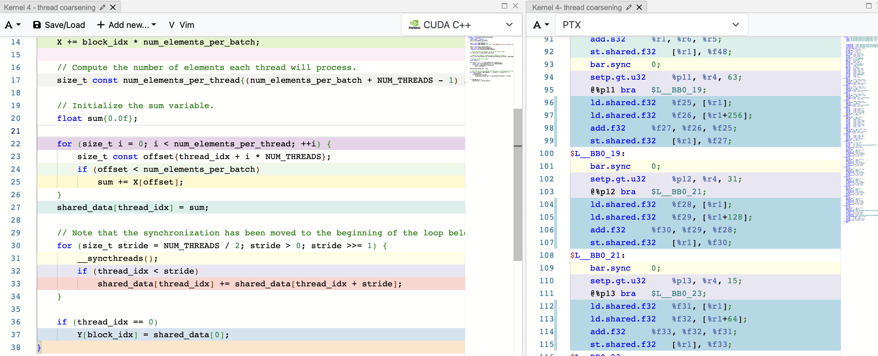
The compiler has already automatically unrolled the for loop in Kernel 4. The PTX code lines highlighted in blue correspond to line 33 in the source code.
To disable this automatic unrolling, we can add #pragma unroll 1 right before the for loop and see the differences in the PTX code.
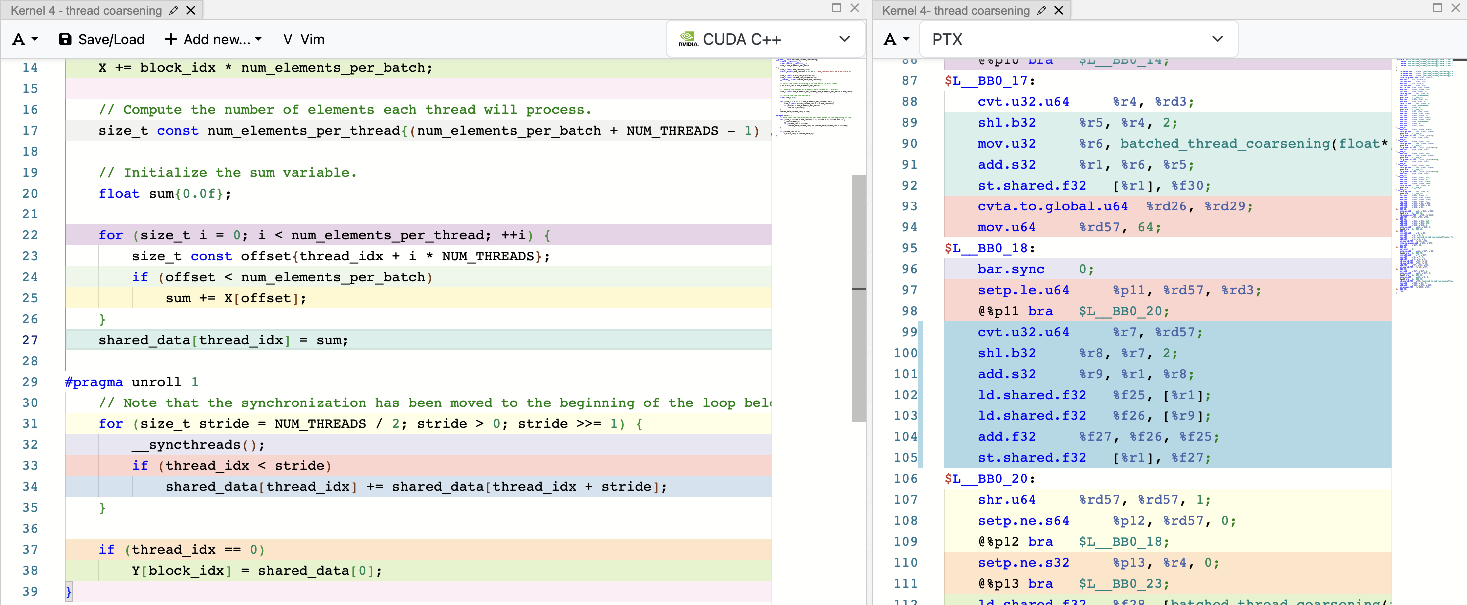
Adding #pragma unroll 1 disables the automatic unrolling. The PTX lines highlighted in blue correspond to line 34 in the source code.
Given this behavior, we can expect no additional performance gain when manually unrolling the for loop.
There is, however, one noticeable difference between Kernel 4 and Kernel 5 version 1 (which unrolls only the last warp). When we reveal the linked code for the lines under warp_reduce() in Kernel 5 version 1, we can see that the following PTX instructions are repeated contiguously (with different memory addresses and registers) without any of the overhead associated with thread synchronization or conditional checks that are present in Kernel 4’s PTX code.
ld.volatile.shared.f32 	%f28, [%r1];      // Load a register variable %f28 from shared memory with address %r1.
ld.volatile.shared.f32 	%f29, [%r1+128];  // Load a register variable %f29 from shared memory with address $r1+128.
add.f32                 %f30, %f29, %f28; // Add %f29 and %f28, then store the result in %f30.
st.volatile.shared.f32 	[%r1], %f30;      // Store %f30 in shared memory with address %r1.
The figure below shows the side-by-side PTX instructions comparison between Kernel 4 and Kernel 5 version 1.
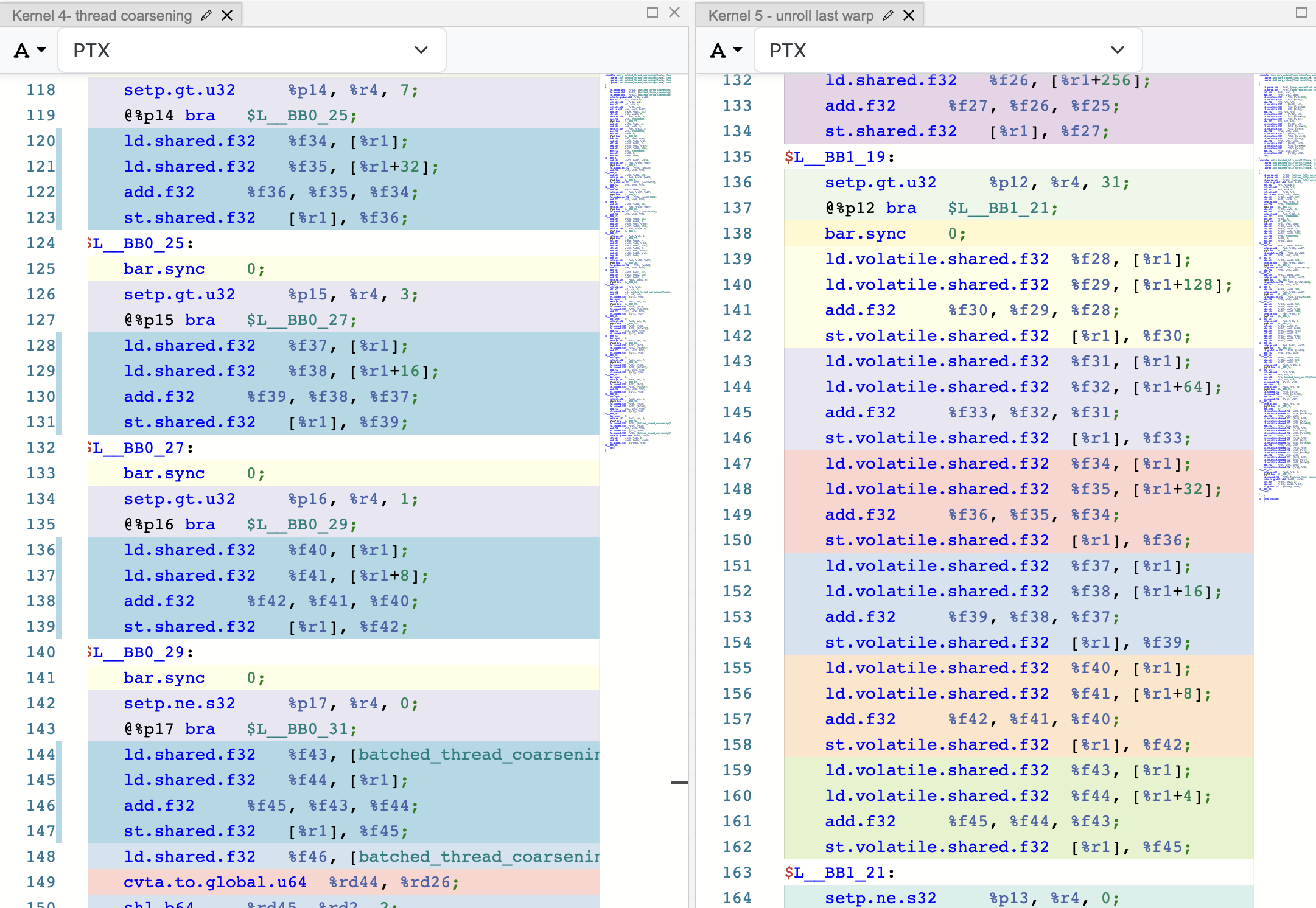
The main difference between Kernel 4 and Kernel 5 version 1.
Even after eliminating instruction overhead, we don’t observe any performance gain. This is likely because the kernel is primarily limited by memory throughput rather than instruction execution.
Obsolete assumption
I mentioned earlier in this section that the changes added to Reduction #5 (or Kernel 5 version 1) are now obsolete on newer GPUs. Specifically, the implicit assumption that threads within a warp execute in strict lockstep is no longer valid starting with Volta architecture. As a result, the modifications made in Kernel 5 version 1 are no longer reliable and may produce incorrect results.
Beginning with Volta (Compute Capability ≥ 7.0), NVIDIA introduced Independent Thread Scheduling: a feature that gives each thread within a warp the ability to execute independently. This change allows developers to explicitly manage intra-warp synchronization using modern mechanisms such as warp shuffle intrinsics or Cooperative Groups.
We will explore the use of warp shuffle intrinsics in the next kernel implementation, as it primarily focuses on fixed warp-level operations. For more information on Cooperative Groups, see this blog.
If You're Curious...
Warp shuffle intrinsics were first introduced in Kepler architecture (Compute Capability 3.x) around five years before Volta. These early versions still assumed implicit thread synchronization within a warp.The Volta architecture later refined this mechanism by introducing the
_sync variants, which include an explicit synchronization mask to support Independent Thread Scheduling. The older intrinsics (those without _sync) were deprecated starting with CUDA 9.0.
>
> For example, __shfl_down_sync() is the modern equivalent of __shfl_down().
Kernel 6: utilizing warp shuffle functions
Recall that in our previous implementations, threads exchanged data using shared memory. Warp shuffle operations allow a thread to directly read a register from another thread within the same warp, enabling threads in a warp to collectively exchange or broadcast data. By using warp shuffle operations, we can reduce shared memory usage, which in turn may allow increasing occupancy when needed.
Additionally, shuffle operations are compiled directly to SHFL instructions in PTX/SASS. This is typically faster than using shared memory, as it effectively only costs a single instruction compared with the minimum of three steps needed for shared memory access (write, synchronize (__syncthreads()), and read). We will look into the instructions in the later part of the section.
To start, Let’s define a new term we haven’t used before in this post: the lane ID. The lane ID is the thread’s index within a warp, ranging from 0 to 31. For example, threads with global indices 2 and 34 both have a land ID of 2 (since thread index % 32 == 2).
In our kernel implementation, the initial setup (e.g., index variable initialization, input array shifting, and summing multiple elements per thread) remains the same as before, except for the size of shared_data. Now, shared_data is allocated with a length equal to the number of warps rather than the total block size, because we only need to store the partial sum from each warp.
    constexpr size_t NUM_WARPS{NUM_THREADS / 32};
    ...
    // The shared data is now among warps rather than threads.
    __shared__ float shared_data[NUM_WARPS];
The rest of the implementation can be divided into the following steps.
1. Obtaining the partial sum from each warp. We’ll be using __shfl_down_sync().
The function __shfl_down_sync() takes four arguments:
unsigned mask: a 32-bit mask indicating which threads in the warp are activeT var: the variable whose value may be accessed by other threadsunsigned int delta: the offset that determines which lane’s value the current thread will readint width: the width of the shuffle group (default is the size of a warp: 32)
This intrinsic allows each lane with ID i to access the value of register var held by the lane with ID i + delta. In other words, it shifts the values of var “down” the warp by delta lanes (the naming was counterintuitive to me; I initially expected it to access the value from lane i-delta instead…). Note the ID number will not wrap around the value of width, so the upper delta lanes will remain unchanged.
The figure below illustrates the following code where we use a shuffle width of 16:
int x = threadIdx.x % 16 + 1;

// All threads are active.
constexpr unsigned int FULL_MASK{0xffffffff};
unsigned int delta = 8;
int width = 16;
int y = __shfl_down_sync(FULL_MASK, x, delta, width);
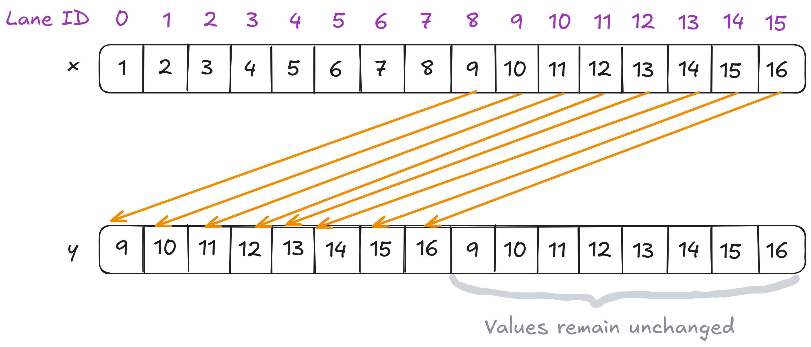
How shuffle down works given a delta of 8 and a group width of 16.
In our code, each lane adds its own sum value to the value of sum held by the lane i + offset, and stores the result back into sum.
    constexpr unsigned int FULL_MASK{0xffffffff};
    for (size_t offset = 16; offset > 0; offset >>= 1) {
        sum += __shfl_down_sync(FULL_MASK, sum, offset);
    }

    // Store the warp element sum in shared_memory.
    if (thread_idx % 32 == 0)
        shared_data[thread_idx / 32] = sum;
    __syncthreads();
We then store the partial sum in the shared memory with index thread_idx / 32.
🚨 CAUTION 🚨
We can safely assume all threads in the warp are active here. In practice, however, we should always perform boundary check to prevent any thread from accessing out-of-bound memory.2. Using the partial sums computed by each warp, we now need to obtain the partial sum for the entire block.
    // Determine active threads for obtaining block sum.
    unsigned int const active_threads_mask = __ballot_sync(FULL_MASK, thread_idx < NUM_WARPS);

    if (thread_idx < NUM_WARPS) {
        // Reuse sum variable to store the shared memory elements.
        sum = shared_data[thread_idx];
        for (size_t offset = 16; offset > 0; offset >>= 1) {
            sum += __shfl_down_sync(active_threads_mask, sum, offset);
        }
    }
The idea is to have each thread read the partial sum produced by the warp whose index matches its own thread_idx. This means that only threads with thread_idx < NUM_WARPS are active in this step. We then perform the same __shfl_down_sync operation as in Step 1 to reduce these warp-level sums into a single block-wide sum.
3. Finally, store the block-wide sum in global memory.
    if (thread_idx == 0)
        Y[block_idx] = sum;
Earlier, I mentioned that warp shuffle operations require only a single assembly instruction. Examining the SASS instruction in Godbolt corresponding to line 34 of the source code (the first __shfl_down_sync()), we see that the first iteration compiles into the following instructions:
 SHFL.DOWN PT, R4, R3, 0x10, 0x1f  // Perform the shuffle.
 FADD R4, R4, R3                   // Add to sum variable.
The performance of all the kernels so far can be found in the table below.
| Kernel # (128 threads/block) |
Mean Effective Bandwidth | % Peak Bandwidth |
|---|---|---|
| kernel 0 | 431.03 | 48.10 |
| kernel 1 | 434.87 | 48.53 |
| kernel 2 | 434.73 | 48.51 |
| kernel 3 | 479.68 | 53.53 |
| kernel 4 | 842.07 | 93.97 |
| kernel 5 | (obsolete) | (skipped) |
| 🆕 kernel 6 🆕 | 841.93 | 93.96 |
Note that we don’t observe any improvement in Kernel 6 compared to Kernels 4. This result is consistent with Lei Mao’s findings: sum reduction is a memory-bound operation, so its performance is primarily limited by memory bandwidth rather than computation.
Nevertheless, it’s still valuable to learn warp shuffle intrinsics, as they are fundamental tools for GPU performance optimization and serve as an excellent foundation for learning and understanding Cooperative Groups.
Kernel 7: vectorized memory access
One final optimization technique I’d like to explore is vectorizing memory loads. Up to this point, our kernels have been loading a single 32-bit register from global memory at a time, as in the statement sum += X[offset];. This compiles into the instruction ld.global.nc.f32 instruction. However, it’s also possible to load larger chunks of data–64 bits or even 128 bits–in a single instruction.
To vectorize our loads, we can use the built-in vector data types. For example, when working with float elements, we can use float4 type, which groups four floating-point numbers together and lets us access them as x, y, z, and w. Using these vector types allows the compiler to generate wider memory load instructions, improving memory throughput and efficiency.
Code-wise, we replace the following:
    // Handle elements of the indices > thread index.
    for (size_t i = 0; i < num_elements_per_thread; ++i) {
        size_t const offset{thread_idx + i * NUM_THREADS};
        if (offset < num_elements_per_batch)
            sum += X[offset];
    }
with
    // Handle elements of the indices > thread index.
    for (size_t i = 0; i < num_elements_per_thread / 4; ++i) {
        size_t const offset{4 * (thread_idx + i * NUM_THREADS)};
        if (offset < num_elements_per_batch) {
            float4 const tmp = reinterpret_cast<float4 const*>(&X[offset])[0];
            sum += tmp.x + tmp.y + tmp.z + tmp.w;
        }
    }
Since we’re now loading four elements at once, we need to adjust both the for loop condition and the offset initialization accordingly. After making these changes, the compiler updates the PTX instruction from ld.global.nc.f32 to ld.global.nc.v4.f32, reflecting the use of a vectorized 128-bit memory load.
This kernel shows a slight improvement compared to Kernel 6:
| Kernel # (128 threads/block) |
Mean Effective Bandwidth | % Peak Bandwidth |
|---|---|---|
| kernel 0 | 431.03 | 48.10 |
| kernel 1 | 434.87 | 48.53 |
| kernel 2 | 434.73 | 48.51 |
| kernel 3 | 479.68 | 53.53 |
| kernel 4 | 842.07 | 93.97 |
| kernel 5 | (obsolete) | (skipped) |
| kernel 6 | 841.93 | 93.96 |
| 🆕 kernel 7 🆕 | 842.22 | 93.99 |
Summary
In this series, we take a deep dive into sum reduction: how it works, how to implement the kernel, and how to further optimize it. My approach builds on Mark Harris’s presentation–which I adapt to take advantage of modern hardware, smarter compilers, and the more recent GPU features–and Lei Mao’s reduction code.
With these optimizations, our kernel hits an effective memory bandwidth of 842.22 GB/s, which is about 94% of the GPU’s peak!
Running the different kernels (excluding the now-deprecated Kernel 5) across various data sizes gives us the following plot. As we can see, Kernel 4 (thread coarsening) stands out with a significant performance boost.
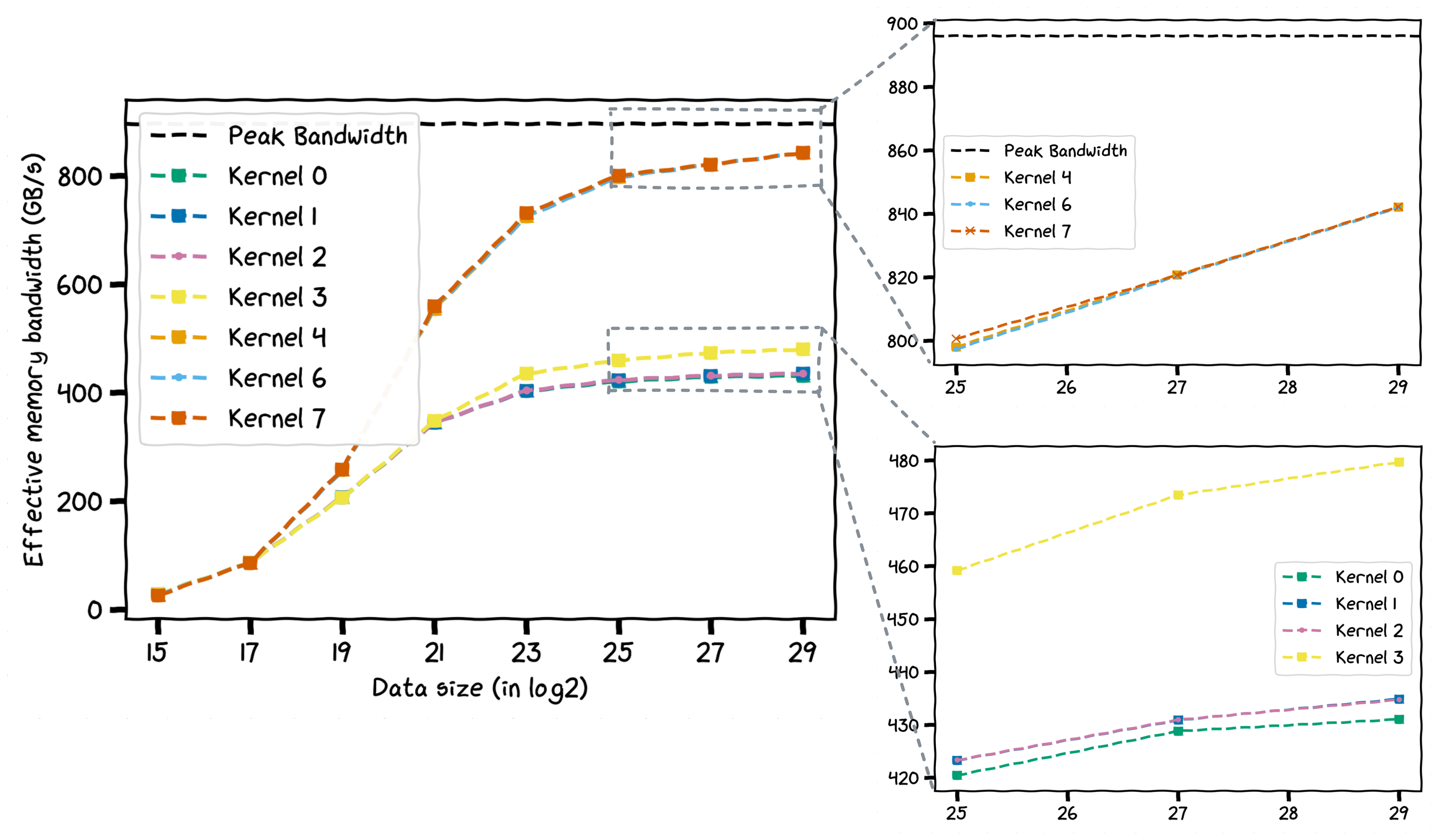
The performance of all kernels across various data sizes.
Resources
- Optimizing Parallel Reduction in CUDA by Mark Harris (2007)
- CUDA Reduction by Lei Mao (2024)
- Programming Massively Parallel Processors, 4th Edition by Hwu, Kirk, and Hajj (2023)
- Dissecting GPU Memory Hierarchy Through Microbenchmarking by Xinxin Mei and Xiaowen Chu (2016)
- Loop Unrolling, Wikipedia
- Faster Parallel Reductions on Kepler by Justin Luitjens (2014)
- CUDA Pro Tip: Do The Kepler Shuffler by Mark Harris (2014)
- Using CUDA Warp-Level Primitives by Yuan Lin and Vinod Grover (2018)
- Godbolt was used for viewing PTX/SASS instructions
- NVIDIA Nsight Compute was used for profiling the kernels
- CUDA C++ Programming Guide
- Illustrations were made with Excalidraw
- The xkcd-style final plot was generated using matplotlib