Bringing PyTorch's Memory Visualizer to MLX
In this post, I will walk through how I implemented a preliminary memory event recorder in MLX where the recorded events can be dumped into a pickle file compatible with PyTorch’s memory viz web app. The main goal of this write-up is mostly to help myself understand what I’m actually doing, as much as I can. If you have any input or feedback, I’d love to hear it!
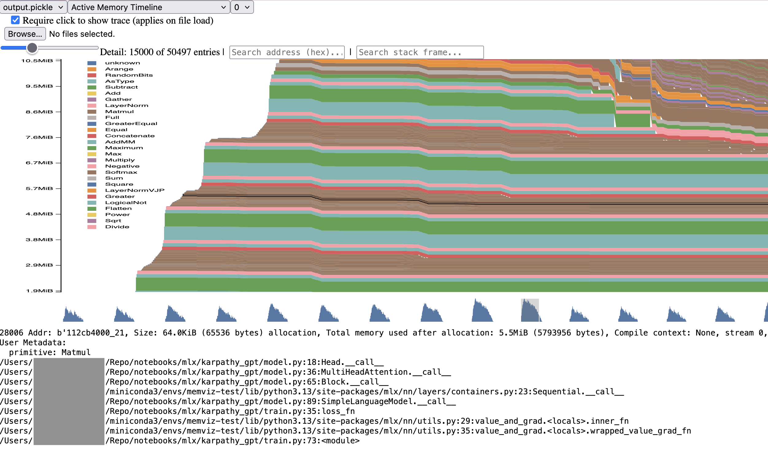
A screenshot example, produced using the code here. Note: if you're wondering why there's nothing allocated in between the iterations, that's because the data is allocated outside of memory recording, and currently, only device_traces is implemented.
The post is organized into the following sections:
- Quick How-To
- Motivation
- The plan
- Plan 1: Understand PyTorch’s side
- Plan 2: Understand MLX’s side
- Plan 3: Bridge the two
- Benchmarks
- Limitations and potential improvements
- Summary
- Appendix
My implementation can be found here.
Quick How-To
To enable memory recording, use the MLX version here and run the following functions:
import mlx.core as mx
from mlx._memory_viz import dump_snapshot

# 1. Turn on the recording.
mx.record_memory_events(enabled=True, max_entries=100000)

# 2. Add things to record.
# ...

# 3. Get the memory events, either:
# 3.1. Get a list of event dictionaries to play around with, or
events = mx.get_memory_events()

# 3.2. Dump the events into a pickle file compatible with PyTorch's memory viz.
dump_snapshot(mx.get_memory_events(), "output.pickle")

# 4. Turn off the recording.
mx.record_memory_events(enabled=False)
Motivation
When learning MLX, I couldn’t find a memory profiler I liked. Maybe I just missed some obvious existing tools out there, but here are two tools I found.
1. MLX's built-in memory API
import mlx.core as mx

mx.get_active_memory() # The number of bytes currently allocated (exclues the buffer cache)
mx.get_cache_memory()  # The number of bytes held in the allocator's reuse cache
mx.get_peak_memory() # THe peak memory mark since program start2. Xcode's Metal Debugger
# run with: MTL_CAPTURE_ENABLED=1 python script.py
mx.metal.start_capture("out.gputrace")   # Path must not already exist
...
mx.metal.stop_capture().gputrace in Xcode. This is a powerful tool, but to my understanding, it's aimed at GPU work (e.g., kernel dispatches) and not at attributing allocations to the lines of code that caused them. It also has a much steeper learning curve.
I really like PyTorch’s memory snapshot visualization where I can record allocation history, dump a pickle, drop it into docs.pytorch.org/memory_viz, and see how each allocation is tied back to the code line that made it. So I decided to build one for MLX. Specifically, to enable MLX output a pickle in a format compatible with PyTorch’s snapshot format so that the existing viewer works out of the box. No new frontend required.
The plan
- Understand PyTorch’s side. How are the memory events recorded? What ends up in the output pickle file?
- Understand MLX’s side. Where does MLX allocate memory? How would lazy evaluation influence the implementation?
- Bridge the two. Output MLX allocation events in PyTorch’s snapshot schema.
I’m new to allocator internals and still learning C++, so I did get assistance from Claude Code, mostly for navigating through unfamiliar codebases, for the C++ I couldn’t yet write unassisted, for correctness verification, and for getting suggestions for relevant readings.
Plan 1: Understand PyTorch’s side
Note: the PyTorch version described here is v2.14.0a0 with head commit 68b353e2. Some details that are deemed irrelevant are omitted.
In PyTorch, we capture memory events using the following functions:
import torch

# Start the recording and set the max capacity of 100_000 entries.
# If there are >100_000 entries, only the *last* 100_000 entries will be stored.
torch.cuda.memory._record_memory_history(max_entries=100_000)

# The training run we want to capture.
...

# Save the snapshot.
torch.cuda.memory._dump_snapshot("out.pickle")

# Stop the recording.
torch.cuda.memory._record_memory_history(enabled=None)
What happens behind the scene?
I’ll divide this section into 4 parts:
- `torch.cuda.memory._record_memory_history(): turning on/off memory event recording
- How trace entries are recorded
torch.cuda.memory._dump_snapshot("out.pickle"): taking a snapshot- Capturing the context
1. torch.cuda.memory._record_memory_history(): turning on/off memory event recording
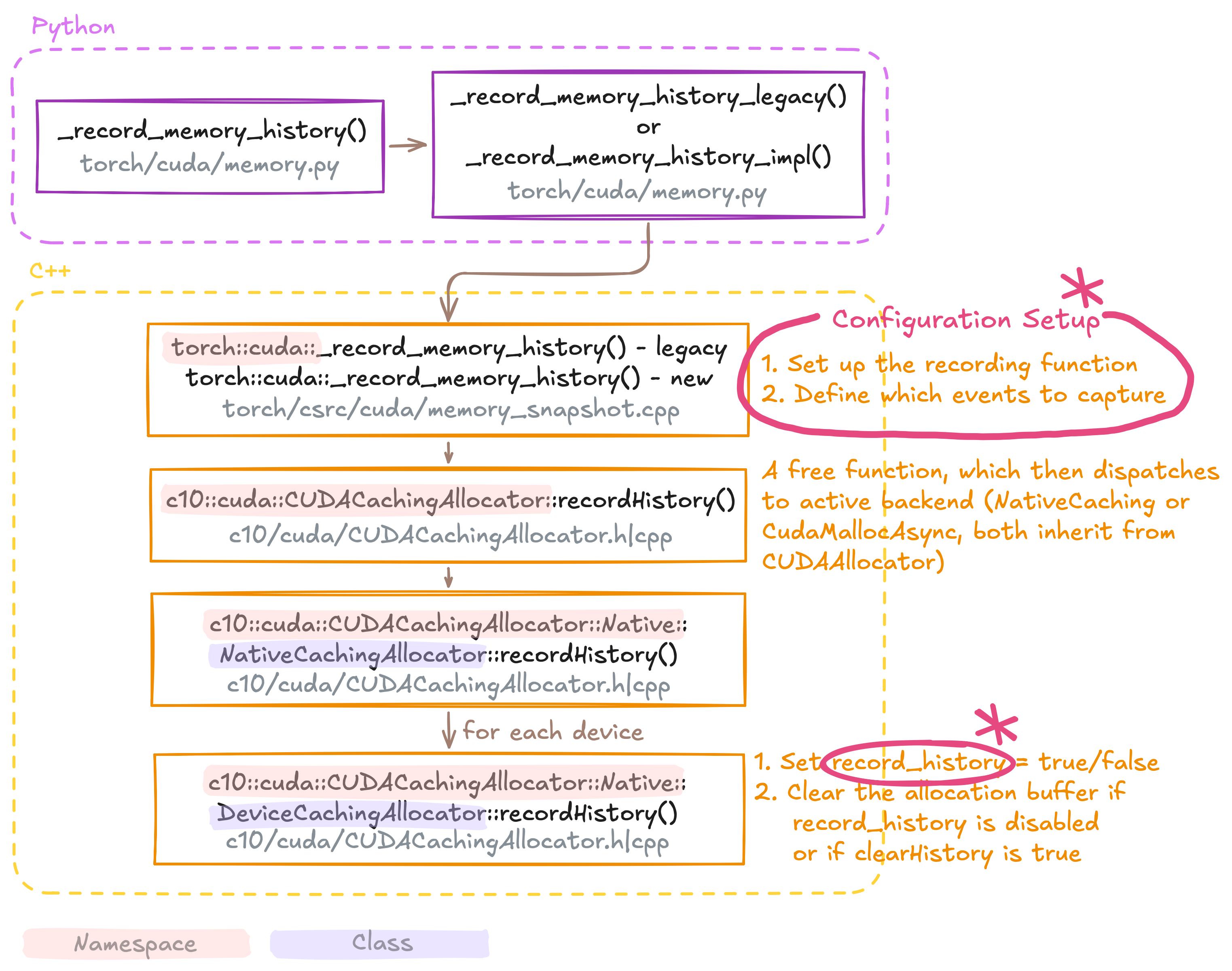
Figure 1. The call path from torch.cuda.memory._record_memory_history() down to the per-device allocator. Note that some details have been omitted for simplicity.
The diagram above may look intimidating, but for our purposes, I’d say torch.cuda.memory._record_memory_history() does two main things (marked with * in the image above):
- Set up the configuration: which context recording function to use and which events to capture.
- Set
record_historyon eachDeviceCachingAllocator.record_historyis a private boolean member ofDeviceCachingAllocator, which is used as the flag the allocator checks later to decide whether to record an event at all.
So no recording happens yet at this point. By default, the enabled argument in torch.cuda.memory._record_memory_history() in the new implementation is set to all, which is then converted into a true value by the time it reaches c10::cuda::CUDACachingAllocator::recordHistory().
2. How trace entries are recorded
All trace entries are captured as TraceEntry objects, created inside record_trace(), a private function on DeviceCachingAllocator. If you search for every record_trace() call site in c10/cuda/CUDACachingAllocator.cpp, you’ll notice they’re called in memory allocation and deallocation paths. The one exception is snapshot(), which records an entry purely as a marker of when the user takes a snapshot. So whenever the user calls a PyTorch function that triggers an allocation or deallocation, record_trace() is invoked.
record_trace() then does the following (with some details omitted):
- Return early if
record_historyisfalseand no trace trackers are registered (I won’t cover trace trackers here.) - Create a
TraceEntryholding the details of the event: its type (allocation, free, and so on), the address, the size, the time it’s created, etc. - If
record_historyistrue, insert the newly created entry into the ring bufferalloc_buffer.
3. torch.cuda.memory._dump_snapshot("out.pickle"): taking a snapshot
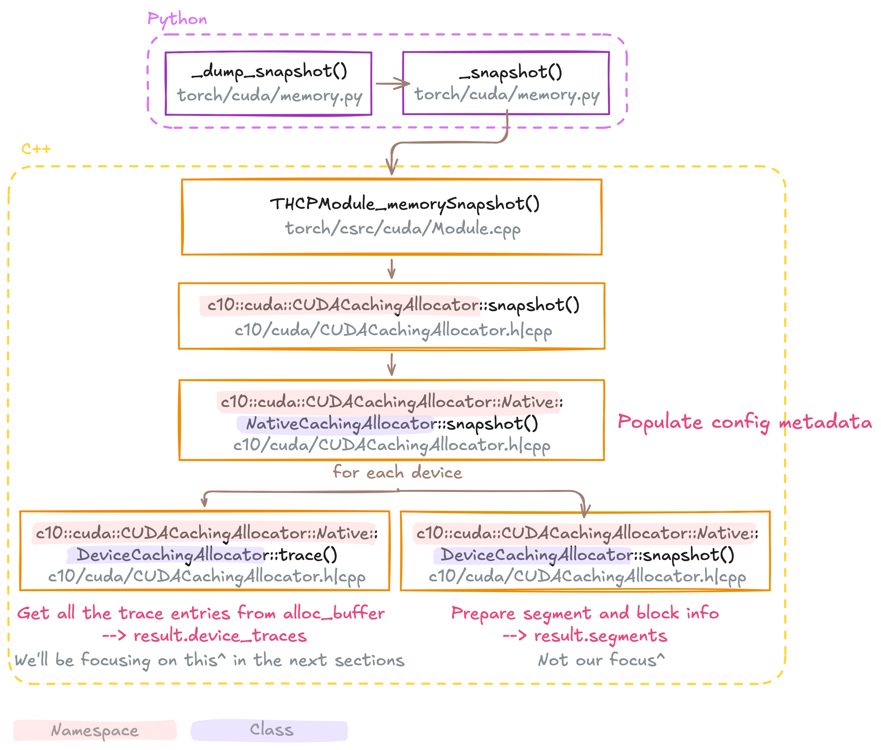
Figure 2. The call path from torch.cuda.memory._dump_snapshot() down to the per-device allocator. Note that some details have been omitted for simplicity.
As you may have expected, the diagram for _dump_snapshot() is very much aligned with _record_memory_history(). Once THCPModule_memorySnapshot() receives the output, it parses the output into a dictionary and passes it back to the Python side. If _dump_snapshot() is called, the dictionary snapshot is then dumped into a pickle file.
Of the two outputs, device_traces and segments, we’ll focus only on device_traces in this post.
4. Capturing the context
One essential component is stack trace capture. Having the call chain that leads to each allocation/deallocation, particularly the Python frames, provides helpful context for debugging. How does PyTorch capture this context? In order to answer this question, I’ll trace the code from the output back to where it’s captured.
The list of {filename, line, name}s comes from TraceEntrys’ context
The docstring of _snapshot() in torch/cuda/memory.py provides clear details of how the memory state is represented. The component we’re interested in is the Frame TypedDict, containing filename, line, and name fields (plus optional FX debug fields, which I will omit in my explanation). Both TraceEntry and Block carry a frames field holding a list of these Frames.
In THCPModule_memorySnapshot(), tracing how the snapshot’s trace_entries is used, we see in traceEntryToDict() that the context comes from the context_ field held by TraceEntry. getCapturedTracebackFromContext(te.context_) returns a raw CapturedTraceback* (I’ll talk more about CapturedTraceback later), which is appended to to_gather_frames. After all entries are processed, the whole batch of frames in to_gather_frames is symbolized at once into filename, line, and name information by py_symbolize(), and the results are written back into each entry’s frames key.
How each TraceEntry’s context is created and passed to record_trace()
Recall that TraceEntrys are created by record_trace(). Tracing where its context argument comes from leads to maybeGatherContext() (one example here). This function loads and invokes context_recorder_, which is the context-recording callback function installed when recordHistory() was called (within the _record_memory_history() call path mentioned in point 1), or returns nothing if recording is disabled, hence the maybe. maybeGatherContext() is called at most once per invocation by the allocator methods that initiate traceable events (e.g., malloc, free, release_blocks, emptyCache).
So now we know when and where “context”s are created and used to create a TraceEntry. But how do we define a “context” to begin with?
What is a “context”?
This is one of the parts I struggled with the most. I hope I’ve understood and explained it correctly, and any feedback is always welcome.
As a member of TraceEntry, context_ is a shared pointer to c10::GatheredContext. GatheredContext itself is defined as an empty polymorphic base (apart from a virtual destructor) on the allocator’s side (c10/core/Allocator.h). Its purpose is to be a type the allocator can access without knowing what’s inside, i.e., an opaque handler (which also means it’s free from any potentially heavy dependencies).
I mentioned CapturedTraceback* very briefly earlier as the type returned by getCapturedTracebackFromContext(). CapturedTraceback inherits GatheredContext and lives on the profiler’s side (torch/csrc/profiler/combined_traceback.h). This is where we see the implementations we’re looking for. Looking at the header, it holds three separate frame vectors: frames_ (Python), cpp_frames_, and script_frames_, and its static gather(python, script, cpp) takes one flag per kind.
Looking back at c10::cuda::_record_memory_history() in torch/csrc/cuda/memory_snapshot.cpp from point 1, we see that the context-gathering callback recorder is set to either gather or gather_with_cpp, which call CapturedTraceback::gather() with the appropriate arguments. recorder is then passed to c10::cuda::CUDACachingAllocator::recordHistory().
If You're Curious...
I had so many questions when I looked at the definition ofGatheredContext for the first time:
// used to hold traceback information in allocators
// ...
struct GatheredContext {
  virtual ~GatheredContext() = default;
};- Ensures clean deletion of the derived class objects.
If an object is deleted through a base class pointer (in our case, aGatheredContext*that points to aCapturedTraceback) and the base class's destructor is non-virtual, the behavior is undefined. In practice, only the base part is destroyed and the derived data members (frames_,cpp_frames_, etc) are leaked. Giving the base class a virtual destructor ensures the entire object is destroyed: the runtime looks up the actual type (CapturedTraceback), runs its destructor first, then the base's.
Though note thatstd::shared_ptrtype-erases its deleter at construction, so since our context here is held usingstd::shared_ptr, the right destructor would run even without thevirtualkeyword.
- Allows the
dynamic_cast<CapturedTraceback*>(x.get())ingetCapturedTracebackFromContext.
At runtime,dynamic_castneeds to know thatx.get()actually points to aCapturedTraceback. But how does it acquire that information?
The moment a class declares any virtual function, it becomes a polymorphic type. In practice, compilers implement this by adding an invisible field, the vptr ("virtual table pointer"), to every object (not the class!) of that class. The vptr points to the class's vtable, which is an array of function pointers used to invoke the appropriate function implementations. The table also contains a reference to the class's type information, the field thedynamic_castuses to determine whetherx.get()points to the right type.
- Effective C++ 3rd Edition, Item 7: Declare destructors virtual in polymorphic base classes, Scott Meyers (2005)
- C++ Virtual Table, Lei Mao (2023)
How are Python tracebacks captured?
Let’s start with python_support_, a linked list of unwinders that is a static atomic pointer to CapturedTraceback::Python. At first, it is initialized as a null pointer in torch.csrc/profiler/combined_traceback.cpp. When import torch is invoked, part of the eager startup registration includes invoking installCapturedTracebackPython() (torch/csrc/profiler/python/init.cpp) and python_support_ is modified such that its head now points to a new PythonTraceback (see the figure below).
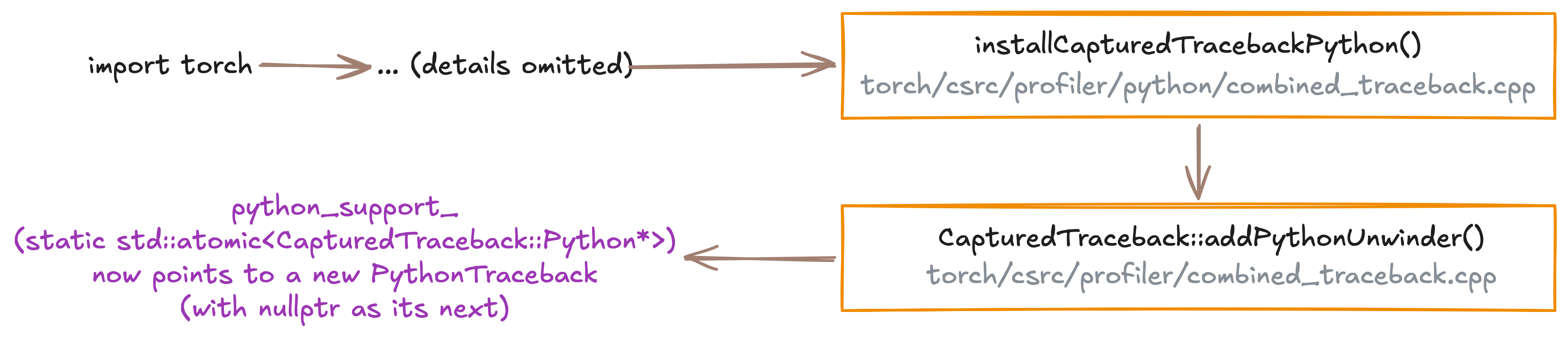
Figure 3. How invoking `import torch` leads to updating python_support_.
When CapturedTraceback::gather() is called with python = True, it walks the unwinder linked list until an unwinder can and does gather Python frames. For each, it first checks PythonTraceback::canGather() (i.e., GIL safety on the current thread). If safe, it calls PythonTraceback::gather(), which gets the current frame via PyEval_GetFrame() and walks up the stack (PyFrame_GetBack()), storing (code, lasti) per frame. Once frames are captured, the loop stops and does not visit remaining unwinders (if any).
I’ll describe how Python frames are handled in PyTorch a bit more when we implement traceback capture.
Plan 2: Understand MLX’s side
Note: the MLX version described here is based on v0.32.1, at head commit 255f953f. Some details that are deemed irrelevant are omitted.
One main thing I learned from PyTorch’s implementation is this: at each memory allocation/deallocation event in the allocator, capture the stack at that moment and attach it to the trace entry as context.
In MLX, we can create a trace entry in the allocation/deallocation path in pretty much the same way, but we can’t capture the traceback there. MLX is lazy, so arrays are only materialized when needed. By the time the allocator actually runs, the Python code that constructed the array has long since returned, so every traceback would point at the eval() line or whatever else that triggers materialization rather than at the code responsible for the allocation.
Before diving into how to resolve this difference, let’s look at the components of MLX that may be relevant for our solution:
I’ll only cover the Metal-backend implementation here for simplicity.
The allocator
MLX currently has a much simpler allocator than PyTorch’s. It has an abstract base class Allocator, which backend-specific allocators derive from (see the figure below).
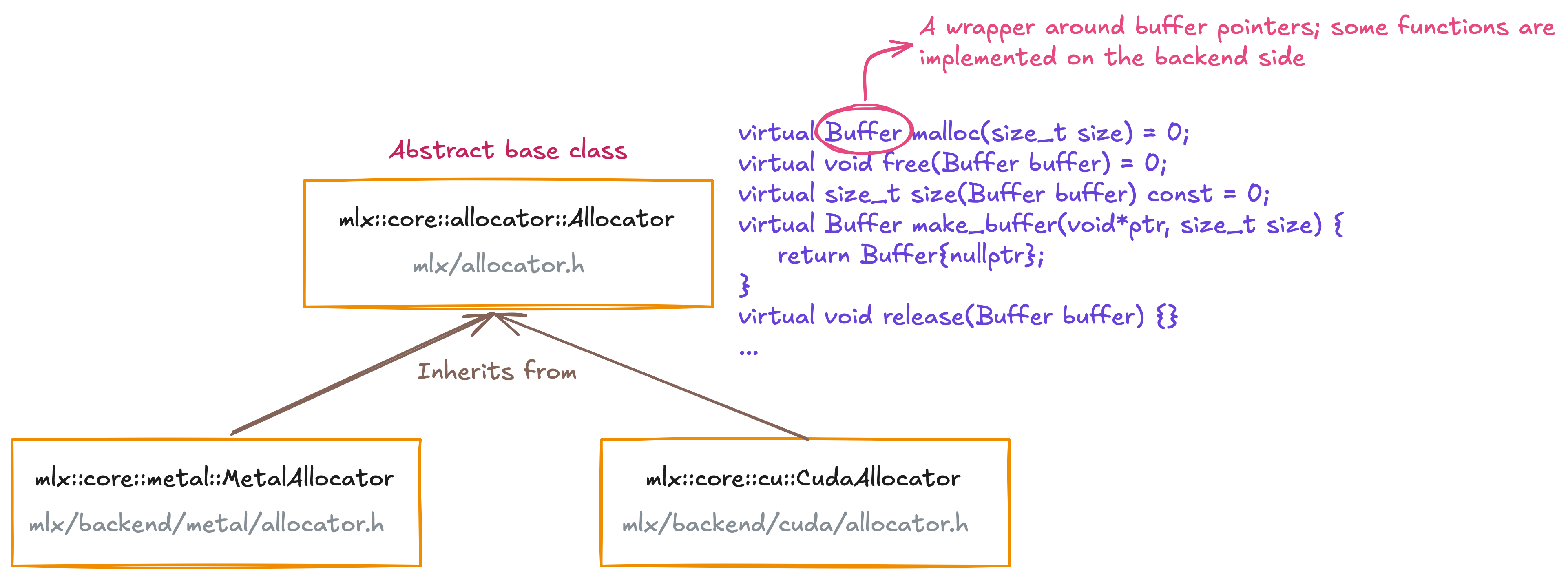
Figure 4. MLX's Allocators.
You might be wondering why there seem to be two sets of allocation and deallocation: malloc/free versus make_buffer/release. Briefly:
mallocandfreehandle buffers that MLX allocates and owns.freeprefers to recycle a buffer into the cache when possible, somalloccan reuse it later.make_bufferandreleasehandle buffers that wrap external memory or foreign raw pointers (e.g., NumPy arrays) without copying. Since MLX doesn’t own that memory,releasetears down the wrapper and never recycles it.
If You're Curious...
What does "recycling a buffer into the cache" means? It's part of what a caching allocator does (which is how MLX implements its allocator, and how PyTorch implements its CUDA allocator as well).Allocating and deallocating GPU memory directly is expensive and slow. To avoid this overhead, the caching allocator keeps freed blocks in the cache instead of returning them directly to the GPU. Then, when a new buffer needs to be allocated, the allocator checks whether the cache has any appropriately sized block to use.
This is why we have the terms active memory and reserved memory. Active memory is the amount of memory currently in use by live arrays (i.e., memory that hasn't been freed yet), whereas reserved memory is the total memory held by the allocator, including active memory and cached (freed but retained) blocks.
Computation graph construction
To have the context point to the right Python line (instead of the line that triggers the eval), our best bet is to place the stack capture somewhere during computation graph construction. So this section aims to identify exactly where.
A computation graph is a directed acyclic graph describing how a result gets computed. Each node is an array object, and an edge from one array to another means the second was computed from the first (as in, the first is the input to the operation that produces the second array). Below is a computation graph example (produced using mx.export_to_dot() before running any mx.eval() implemented in mlx/graph_utils.cpp) along with the computation code.
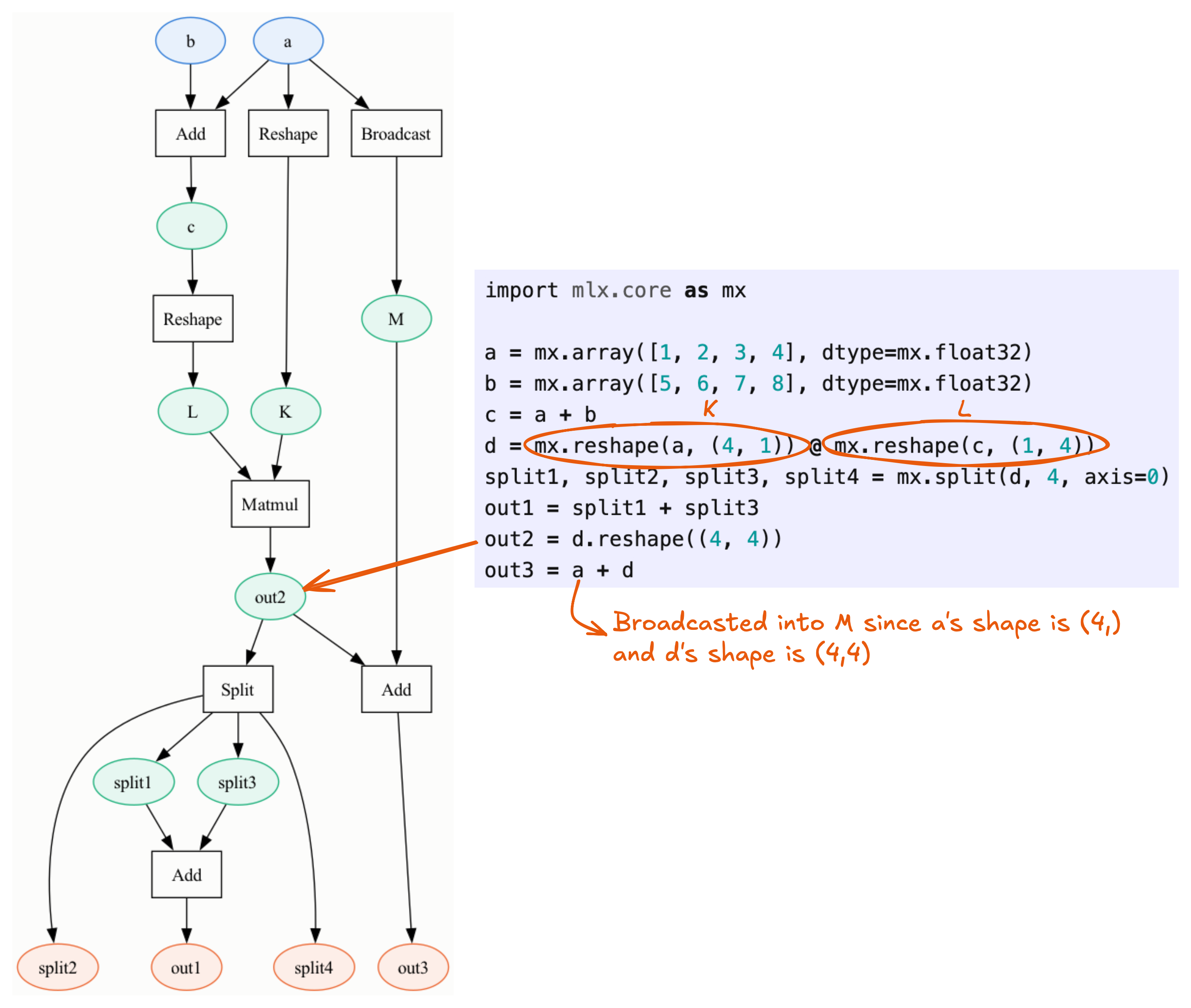
Figure 5. A computation graph example.
How is the graph constructed? What happens when we invoke each of the line in the example code above? To answer the questions, we’ll start by delving into the class array.
The array class (and its nested ArrayDesc struct)
As mentioned in the docstring, “an array is really a node in the graph”. Looking at its private member, it actually only holds a shared pointer to ArrayDesc object, array_desc_. An array is therefore just one pointer wide, which is what makes passing it around by value cheap. Most of its public functions are thin accessors that forward to the data contained within array_desc_.
Looking at the ArrayDesc struct definition, we see the following information:
- The metadata: shape, strides, size, dtype, offset, data_size (how many elements of the buffer it actually accesses), flags (contiguity information).
- The operation: a
std::shared_ptr<Primitive> primitive, which knows how to compute the array’s data from its inputs. For leaf arrays, the primitive would be null. - The status, which is one of:
unscheduled: the computation producing the output array has not been scheduled yet.evaluated: the array’s evaluation has been run, but the computation is not necessarily complete. Its memory has been allocated, and if the array is not a tracer, it has been detached from the graph (with its primitive and inputs dropped) so the upstream graph can be freed.available: if the array is the output of a computation, then the computation is complete and the data is safe to read.
- The event: a handle to the completion signal for the operation that produces this array’s data. It is what promotes an array fom
evaluatedtoavailable. - The tracer flag (
is_tracer): marks an array that is being used inside a graph transform such asgradorcompile, and so must not be detached from the graph at eval time. - The data: a
std::shared_ptr<Data>, whereDatais the buffer along with its deleter. - The inputs: the inputs to the operation held by the array
- The siblings: the co-outputs of a multi-output operation, along with
position, this array’s index in that output list.
There are multiple possible levels of sharing here:
- Multiple
arrayhandles sharing oneArrayDescare the same array. Also notice thatid()of the array returns the address of that sharedArrayDescobject, so these handles all report the sameid(). - Multiple
ArrayDescs sharing oneDataare different views onto the same memory, each with its own shape, strides, and offset. - Multiple
ArrayDescs sharing onePrimitiveindicate the co-outputs of the same multi-output operation
I will show examples of each in the section below.
What happens when we run each line in the Fig. 5 example?
Now that we know what array is, we can look into what the lines in the example code actually do. Let’s start with the following lines.
a = mx.array([1, 2, 3, 4], dtype=mx.float32)
b = mx.array([5, 6, 7, 8], dtype=mx.float32)
Each line above calls create_array(), which is defined in python/src/convert.cpp. Tracing it through a few more layers eventually reaches return mx::array(vals.begin(), shape, dtype);. It calls one of array’s constructor, which initializes array_desc_ via ArrayDesc’s constructor and its init() function. Notice that these leaf arrays are immediately available, i.e., the data is materialized right away and no evaluation is needed. So a question worth to think about: would leaf arrays need a separate method to capture the stack?
c = a + b, on the other hand, invokes a.__add__(b), which calls mx::add(a, b) that is defined in mlx/ops.cpp. It in turn calls an array’s constructor, an ArrayDesc’s constructor, and invokes ArrayDesc’s init().
.reshape() is an interesting one since it can behave in several ways. mx.reshape(a, (4, 1)) (producing node K in the figure) and mx.reshape(c, (1, 4)) (node L) follow paths similar to the operations above, ending in the array and ArrayDesc constructors. Note that creating a new array and array_desc_ doesn’t necessarily mean memory gets allocated at eval time. During eval, MLX first checks the input’s layout. A row-contiguous input always yields a view, otherwise MLX still tries to express the new shape as strides over the existing buffer. It only copies as the last resort. When a view is produced, the new ArrayDesc points to the same data instead of allocating a new buffer (recall the third level of sharing mentioned above). To repeat, a node/array creation doesn’t always lead to memory allocation.
out2 = d.reshape((4, 4)), on the other hand, behaves differently. You might have noticed d is missing in the figure! What happened to d? By this point, d’s shape is already (4, 4), so reshape() function simply returns d by value, copy-constructing a new handle. out2 and d are therefore two different array handles sharing one ArrayDesc (the first level of sharing above).
One other operation I’d like to highlight is split(), which produces multiple outputs (i.e., generating new array objects with their own ArrayDescs) that share a single split primitive (the second level of sharing above). Each output holds references to the others as its siblings.
In summary, array-related Python operations that may(!!!) end up with allocations all pass through ArrayDesc’s init(). It runs while Python frame that created the array is still on the stack. Several other important things include:
- We may need to capture the traceback separately for leaf arrays.
- A node/array creation does not always lead to memory allocation.
- (Not discussed above) A single operation may lead to multiple nodes being created. For example, when broadcasting is needed to run an operation, it creates one node for the broadcast and another for the operation itself.
What happens when eval is triggered
When we run mx.eval(out1, out2, out3) at the end, it passes through these lines before reaching the core function eval(). As long as there’s any unscheduled graph work, it calls eval_impl() and waits for it to finish.
eval_impl() starts by wrapping the outputs the user asks for in a synthetic Synchronizer node (sync below), giving the graph a single root to traverse from. It then does three things:
-
Compute the out-degree (i.e., the number of consumer of each node in the graph) using depth-first search (DFS). For the example above:
| Node | Out-degree | Consumer nodes | Primitive | |----------|------------|--------------------|-----------| | a | 3 | c, K, M | leaf | | d (out2) | 3 | split*, out3, sync | Matmul | | split1-4*| 2 | out1 | Split | | K | 1 | d (out2) | Reshape | | L | 1 | d (out2) | Reshape | | M | 1 | out3 | Broadcast | | b | 1 | c | leaf | | c | 1 | L | Add | | out1 | 1 | sync | Add | | out3 | 1 | sync | Add | *siblings share a single count. out1 has split1 and split3 as its inputs. -
Build the tape, a deque holding the order in which operations run, so that every producer runs before its consumers and each operation runs exactly once. The tape is built with breadth-first search (BFS). The example above generates:
tape: [sync, out1, out3, split3, M, d (out2), K, L, c] execution: c --> L --> K --> d (out2) --> M --> split3 --> out3 --> out1 --> sync -
Run the operations in the tape. Each primitive is invoked in these lines, and that is where output buffers are allocated.
Plan 3: Bridge the two
Recall that in PyTorch, whenever recording is enabled and it’s GIL-safe (i.e., when the thread legally holds the GIL), the Python stack is gathered synchronously during the alloc/free call and passed to the trace-recording function placed in the allocator.
In MLX, however, while it’s still straightforward to place the recording function in the allocator, its lazy computation design means the Python context has to be captured separately. This is because by the time the allocation happens, the Python frame that created the array is long gone. One idea is to capture the context during graph construction instead. As discussed earlier, array-related Python operations that may end up with allocations all pass through ArrayDesc’s init(), so we can record the context there and carry it on the array descriptor array_desc_, then to be picked up by the memory trace entry when the buffer is eventually allocated.
Here are the implementation steps. My main goal at this point is a working prototype, so I’m not worrying much about optimization, and I might overlook some details. Some naming may also change in the future.
- Enable recording memory events.
- Capture the primitive name associated with each event.
- Implement traceback capture.
- Format the output to match PyTorch’s snapshot format.
While my earlier descriptions referenced a specific commit of MLX (and PyTorch), my implementation is based on the commit tagged as the latest MLX release a the time (v0.32.1)
1. Enable recording memory events.
This step is fairly straightforward and it entails the following substeps:
- [C++ Backend] Implement a recording function, along with a class representing a memory event, and call it from the allocator’s allocation and deallocation paths.
- [C++ Backend] Ensure the memory event class contains a flag to indicate whether the recording is enabled or not.
- [Python-facing] Provide a functionality to toggle the recording functionality (similar to PyTorch’s
_record_memory_history()). - [Python-facing] Expose the captured events to Python (for testing purposes).
2. Capture the primitive name associated with each event.
Since we’re not capturing C++ stacks, the primitive names carry most of the signal about where an allocation came from.
To record which primitive an allocation/deallocation belongs to, we need to get the primitive’s name from array down to the event recording function. Recall from the eval description section that primitives are invoked in these lines where arr is passed to either gpu::eval() or cpu::eval().
One solution is to thread the name through the call path, passing it alongside arr all the way down to where memory is allocated or freed. The problem is that the call path can get tedious, so plumbing an extra argument through every branch that might allocate/deallocate gets messy pretty fast…
Another solution is to create a context object: an object that stores information at one point in the call stack so it can be read further down without being passed explicitly. We Implement two structs in mlx/op_context.h:
struct OpInfo {
  std::string_view primitive_name;
};

inline thread_local OpInfo current_op;

struct OpContext {
  explicit OpContext(std::string_view primitive_name) {
    current_op = {.primitive_name = primitive_name};
  }
  ~OpContext() {
    current_op = {};
  }

  OpContext(const OpContext&) = delete;
  OpContext& operator=(const OpContext&) = delete;
};
We can then set the primitive name right before gpu::eval(arr) or cpu::eval(arr) and read it back inside the memory event recording function. That way, the allocator is able to pick it up no matter how deep the call path goes.
3. Implement traceback capture.
Possibly the most challenging part of the implementation for me. I relied heavily on Claude Code for this one due to my lack of experience.
Challenges
In both PyTorch and MLX, there is a Python layer and a C++ layer. The allocator runs in pure C++ and handles allocations, deallocations, and memory event recording. Meanwhile, we want to capture Python stacks and attach the captured PyObjects to the recorded memory event. Here is the catch: the allocator cannot include Python headers (i.e., cannot use PyObject). PyTorch solves this with the three layers illustrated in Figure 6 below.
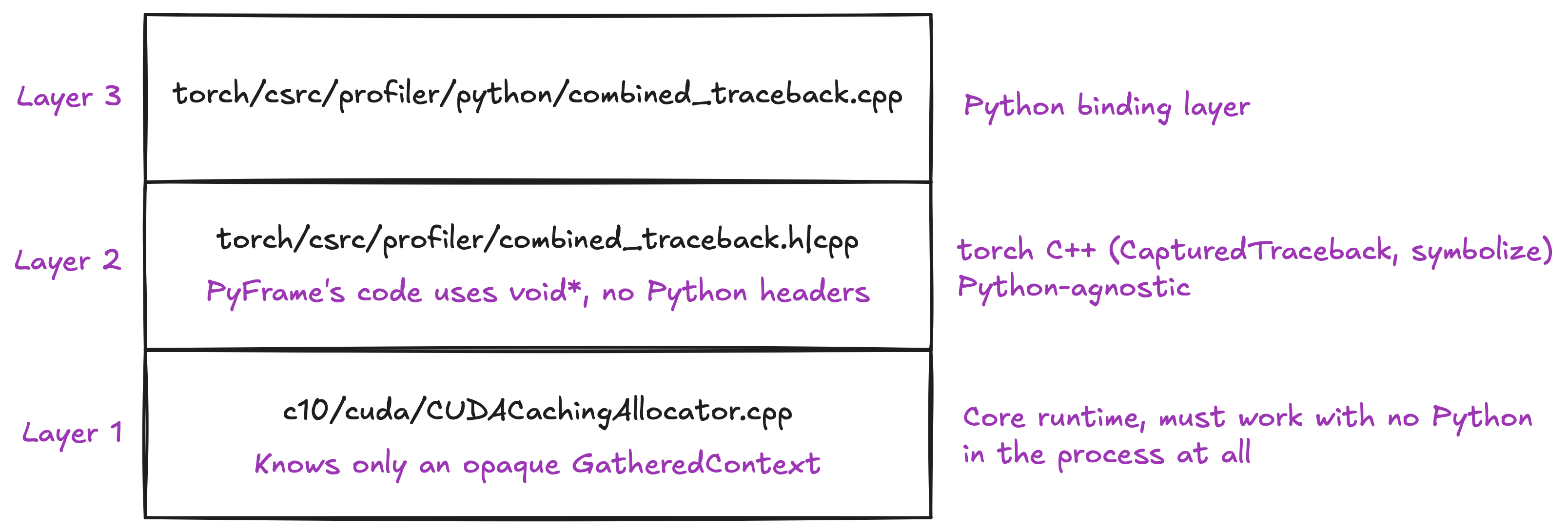
Figure 6. The layering design in PyTorch.
- Layer 1: The allocator sees only an opaque
GatheredContextand invokescontext_recorder_(which we discussed earlier) to produce one. - Layer 2: torch C++ sees the
PyFrametype, which stores the frame’s code object as avoid*rather than aPyObject*. Avoid*can be stored, moved, and compared, but never dereferenced, meaning, this layer cannot INCREF, DECREF, or read a filename. Anything that needs to interpret the pointer goes through a virtual interface that Layer 3 registers at import time. - Layer 3: The Python binding file, which implements all the Python-specific operations, from walking the frame stack, resolving frames to filenames and line numbers, to releasing references.
If You're Curious...
Py_INCREF() and Py_DECREF() are Python C APIs for managing an object's reference count. When Py_DECREF() brings the count to zero, it immediately invokes the object's deallocator, which releases the object.
Here is where the problem lies. Layer 2 owns strong references to code objects but cannot safely release them. Releasing means Py_DECREF, which may only be called when holding the GIL, and ~CapturedTraceback can run on a thread that is currently holding the allocator’s device lock. Acquiring the GIL there can deadlock (explained in the comments here): one thread holds the GIL and waits for the device lock, while another holds the device lock and waits for the GIL. So instead of freeing immediately, PyTorch implements it such that the destructor defers. It pushes the doomed frame pointers onto a global to_free_frames vector. The actual Py_DECREFs happen at the top of the next gather() call, which by construction holds the GIL and runs outside the device lock.
Solution
To mitigate this problem, instead of passing the PyObject* (in the form of void*) to the allocator, we can intern each captured stack in a table on the Python side and pass an integer ID into the memory event recording instead. The table owns the only references to the code objects and never releases them during a session, so destroying a memory event just destroys an integer (no Py_DECREF and no GIL).
This entails the following steps:
-
In
mlx/traceback.h|cpp, implement the hook mechanism:set_traceback_tracking()to toggle tracking,set_traceback_capture_func()to install the capture hook (which is invoked byinstall_traceback_capture()), andcapture_traceback()to invoke the hook.capture_traceback()returns aTracebackId, and the core only transports it. -
Add a new
ArrayDescfieldtracebackfor storing the traceback ID. - Capture the traceback when the
ArrayDescis created (we discussed earlier how theinit()function can be a reliable capture point):void array::ArrayDesc::init() { ... traceback = detail::capture_traceback(); } -
Add the traceback ID to
OpInfo, so the thread-localcurrent_opcan carry it from the eval loop to the allocator. -
Pass the array’s traceback ID when constructing
op_contextintransforms.cpp. -
Add a traceback ID field in
MemoryEvent. - Call
set_traceback_tracking(enabled)inrecord_memory_event()(next to the existingset_op_tracking(enabled)), and attach the traceback inmaybe_record_events():if (MemoryEvent::is_alloc(action)) { event.primitive_name = detail::current_op.primitive_name; // Add the lines below. event.traceback = detail::current_op.traceback != detail::no_traceback ? detail::current_op.traceback : detail::capture_traceback(); }The fallback in the last line exists for leaf arrays. Leaf arrays allocate eagerly at construction without
eval(), so noOpContextever runs andcurrent_opcarries no ID. Consequently, the ID sitting inArrayDescis unreachable from the allocator, whose interface is justmalloc(size). But leaf construction happens on the Python thread with the GIL held, so the allocator can simply capture directly. This is safe because the capture function never attempts to acquire GIL; it only checks if GIL is held. In other use cases (the eval path), the check fails and the fallback harmlessly returnsno_traceback(thoughcurrent_opalready has the ID anyway). -
Implement the capture function itself in
python/src/traceback.h|cpp, along with the interning table. For deduplication, the table hashes each captured stack. I picked the Fowler–Noll–Vo hash for its simplicity and for how easily it folds frame by frame into a running hash. - Also in
python/src/traceback.h|cpp, implementresolve_traceback(TracebackId id), which turns an ID back into a readable stack: a list of(filename, function name, line number)tuples, ordered outermost frame first to match Python’s own traceback convention. This is called from theget_memory_events()binding.
4. Format the output to match PyTorch’s snapshot format.
PyTorch’s snapshot dictionary contains the following fields: segments, device_traces, allocator_settings, external_annotations, host_segments, and host_traces. For our first prototype, we’ll only include device_traces and segments. Specifically, we’ll implement device_traces and leave segments as an empty list.
Since we already have mx.get_memory_events(), we just need a function that reformats its output into a form the memory viz web app can load. Note that we want to handle two different timelines:
- Active memory: the memory arrays are actually using right now.
- Allocation actions:
{"AllocNew", "AllocReuse", "AllocMakeBuffer"}, to be replaced withalloc - Free actions:
{"FreeActiveToCache", "FreeActiveToOS", "Release"}, to be replaced withfree_completed
- Allocation actions:
- Reserved memory: the memory taken from the OS that hasn’t been released yet, i.e., active memory + what’s retained in the cache
- Relevant allocation actions:
{"AllocNew", "AllocMakeBuffer"}, to be replaced withsegment_alloc - Relevant free actions:
{"FreeActiveToOS", "Release", "FreeCacheToOS"}, to be replaced withsegment_free
- Relevant allocation actions:
Since I don’t currently capture C++ stacks, the primitive name carries most of the useful signal. In my current implementation, primitives are used as event categories, which the viewer displays as graph colors and legend entries. The problem is that there’s only a limited number of colors, so distinct primitives end up sharing one. To work around this, I also added the primitive name to the user metadata, where it shows up as text (shown in the figure below).
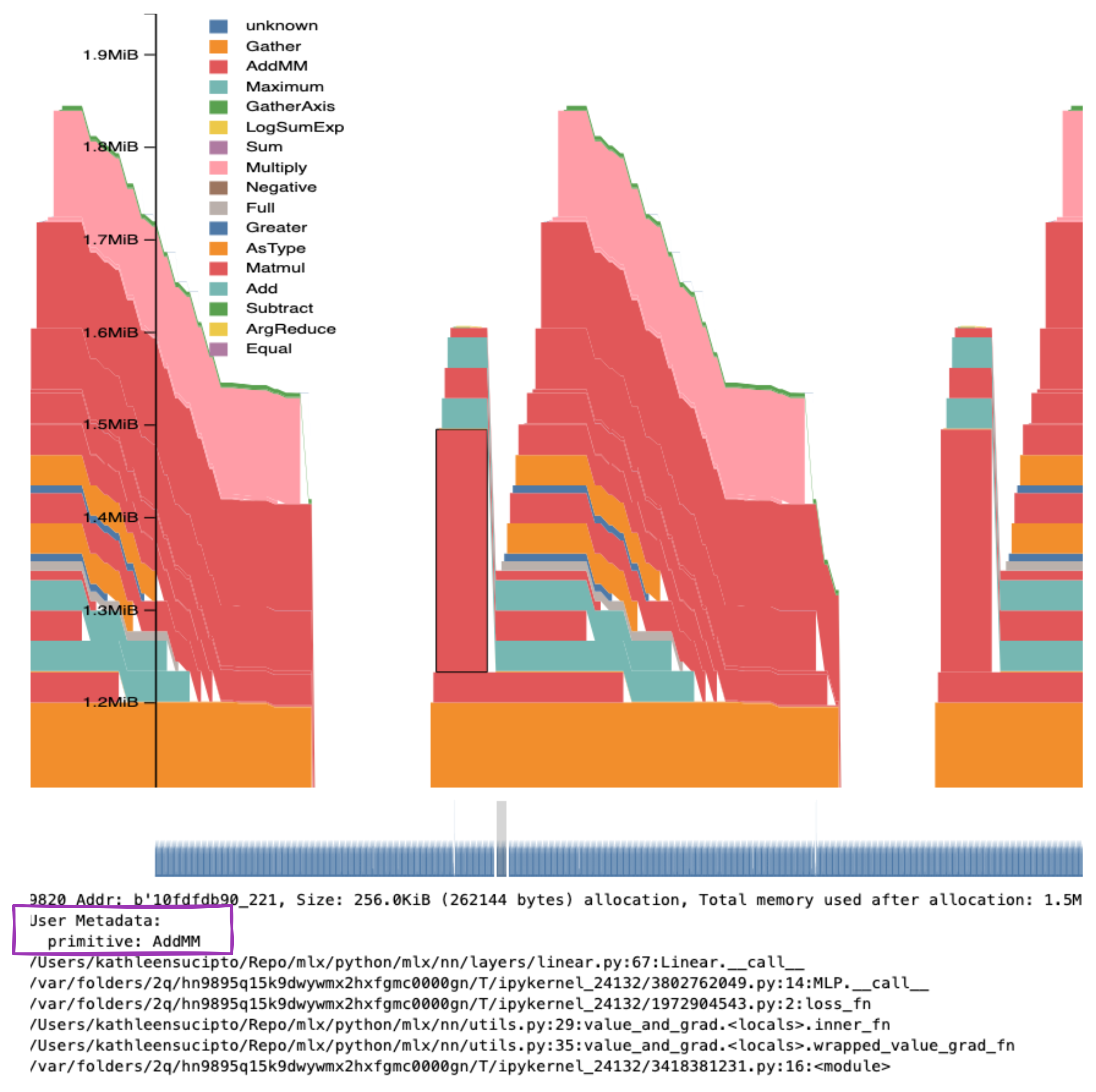
Figure 7. User metadata displayed on memory viz.
Benchmarks
To assess the performance of the memory event recording functionality, I ran two kinds of benchmarks on an M3 MacBook Air (16 GB unified memory, macOS Tahoe 26.5.2):
- Estimating the cost of having the functionality implemented, i.e., comparing no functionality vs. with functionality (recording off)
- Assessing the performance of stack capture and event creation
1. Estimating the cost of having the functionality implemented
Both Python stack capture and event creation are only performed when the recording is on. When the recording is disabled, however, the following still happen:
- The invocation of
capture_traceback()when initializing an array (which returns early if recording is disabled). - When eval is invoked:
- The atomic load of
op_tracking_enabledand the call to theOpContextconstructor, which retrieves each array’s primitive name and traceback ID. - The invocation of
maybe_record_events()(which returns early if recording is disabled) in every allocation and deallocation.
- The atomic load of
We don’t want these steps to add noticeable cost. To measure this, I added two Python benchmark functions below.
def benchmark_full():
  val = mx.array(10.0)
  mx.eval(val)

  def run_benchmark():
    outs = []
    num_iters = 3 # update with either [1, 2, 3].

    def recursive_op(i, outs, val):
      # To ensure full 32 frames, explained in the next benchmarks.
      if i == 31:
        x = mx.full((10, 10), val)
        outs.append(x)
      else:
        i += 1
        recursive_op(i, outs, val)

    for _ in range(num_iters):
      for _ in range(10):
        recursive_op(0, outs, val)
    return outs

  # From time_utils.
  time_fn(run_benchmark)

def benchmark_add():
  val = mx.full((10, 10), 10.0)
  mx.eval(val)

  def run_benchmark():
    outs = []
    num_iters = 3 # update with either [1, 2, 3].

    def recursive_op(i, outs, val):
      # To ensure at least full 32 frames, for the next benchmarks.
      if i == 31:
        x = val + val
        outs.append(x)
      else:
        i += 1
        recursive_op(i, outs, val)

    for _ in range(num_iters):
      for _ in range(10):
        recursive_op(0, outs, val)
    return outs

  time_fn(run_benchmark)
Notice the tiny array size. Since event and array (relevant for stack capture) counts are independent from array size, shrinking the size would help maximizing the overhead’s visibility by collapsing the per-op baseline. Each op runs 1000 times per batch across 50 batches. Some warmup steps are also run beforehand. Additionally, the benchmark was run on the CPU since the scheduling and synchronization cost in the GPU may end up swamping the effect being measured.
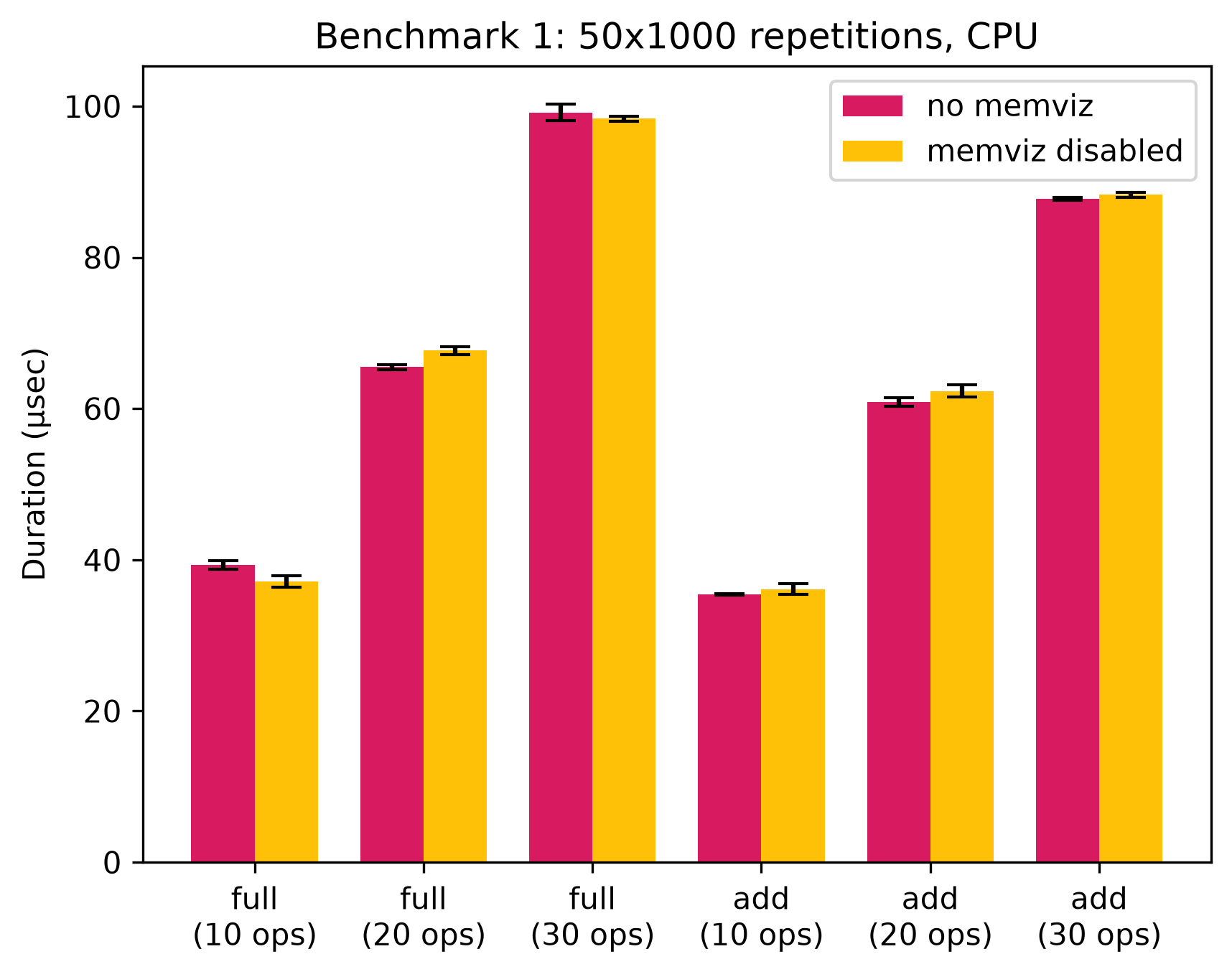
Figure 8. Benchmark 1 results. no memviz represents the original MLX code (v0.32.1) and memviz disabled represents MLX v0.32.1 + memory event recording implemented but disabled. The error bars represent 95% confidence interval.
In the plot above, we see that the memviz disabled bars are not consistently higher than the no memviz bars. The differences between adjacent bars are also so tiny that they could be mainly attributed to noise.
You might also notice that the full operation takes longer than the add operation. This is because the full operation actually constructs two arrays/nodes in the computation graph: one from broadcast, to reshape val from () to (10, 10), and the other from the full operation itself. Meanwhile, add only constructs one node. This detail will become more important in the next benchmark.
In summary, according to this benchmark result, adding the memory event recording implementation does not seem to introduce any noticeable extra cost.
2. Assessing the performance of stack capture and event creation
When memory event recording is enabled, recall that the Python stack is captured during graph construction and the memory events are captured when eval is triggered. Specifically,
- For each node creation in the graph:
- Invokes
capture_traceback(), which captures the Python stacks with a maximum depth of 32 frames - Interns the stack
- Invokes
- When eval is invoked:
- Atomic loads
op_tracking_enabledand creates (and destroys)OpContext, which retrieves each array’s primitive name and traceback ID during creation - Invokes a complete
maybe_record_events()in every allocation and deallocation
- Atomic loads
In this benchmark, we hope to measure the cost of 1) each stack capture (including the stack interning) and 2) the event creation. To do so, we run the same benchmark functions above with memory event recording on and off, once with no eval invocation and once with eval. The recursive function call is implemented to reach 32 frames, which is the maximum number of walks during stack interning. The results can be found in the table below.
Durations [95% CI intervals] of full operations, along with computed stack-capture and event-creation costs (all in μsec), 50 × 1,000 repetitions
| eval invoked | # Ops | # Ops Events* | memviz disabled |
memviz enabled |
Cost of stack capture | Cost of event creation |
|---|---|---|---|---|---|---|
| No | 10 | 0 | 14.763 [14.682, 14.845] | 50.314 [50.151, 50.478] | 1.777 | - |
| Yes | 10 | 1M | 37.174 [36.411, 37.936] | 76.840 [75.864, 88.815] | NC | 0.206 |
| No | 20 | 0 | 30.184 [29.319, 31.049] | 100.193 [99.661, 100.725] | 1.750 | - |
| Yes | 20 | 2M | 67.668 [67.108, 68.228] | 137.640 [136.068, 139.213] | NC | -0.002 |
| No | 30 | 0 | 44.386 [44.258, 44.514] | 146.574 [146.085, 147.062] | 1.703 | - |
| Yes | 30 | 3M | 98.336 [97.976, 98.697] | 191.888 [191.233, 192.543] | NC | -0.288 |
Table remarks:
NC=Not computed# Ops Eventshere includes the events created across all batches and iterations. Recall that we repeat the function 50 × 1,000 times. If there are 1 million events created, then each op creates $(1,000,000 / 50,000) / 10\ ops = 2\ events/op$.
To compute the cost of each stack capture, we can use the following formula:
\[t_{each\_stack\_capture} = \frac{(t_{memviz\_enabled\_no\_eval} - t_{memviz\_disabled\_no\_eval})}{\#\ arrays\ created}\]For instance, the cost of each stack capture given 10 full operations would be:
The denominator comes from 10 operations multiplied by two arrays constructed in each operation.
As for the cost of an event creation, we can use the following formula:
\[t_{each\_event\_creation} = \frac{(t_{memviz\_enabled\_with\_eval} - t_{memviz\_disabled\_with\_eval}) - (t_{all\_stack\_captures})}{\#\ events}\]where \(t_{all\_stack\_capture} = t_{memviz\_enabled\_no\_eval} - t_{memviz\_disabled\_no\_eval}\)
So the cost of an event creation given 10 full operations would be:
Computing the rest would lead to the values shown in the table above. Based on the results, I found that while the cost of each stack capture is comparable (roughly 1.8 μsec), the cost of each event creation is all over the place. To investigate, I ran some C++ benchmarks (which means no Python traceback capture function is installed) and found that the cost of each event creation seems almost negligible and is mostly affected by noise (see Appendix).
Running the same benchmark method on the add op lead to similar results.
Durations [95% CI intervals] of add operations, along with computed stack capture and event creation costs (all in μsec), 50 × 1,000 repetitions
| eval invoked | # Ops | # Ops Events | memviz disabled |
memviz enabled |
Cost of stack capture | Cost of event creation |
|---|---|---|---|---|---|---|
| No | 10 | 0 | 13.741 [13.668, 13.815] | 31.403 [31.311, 31.495] | 1.766 | - |
| Yes | 10 | 1M | 36.135 [35.415, 36.855] | 56.372 [55.325, 57.418] | NC | 0.129 |
| No | 20 | 0 | 26.955 [26.733, 27.177] | 62.286 [62.116, 62.455] | 1.766 | - |
| Yes | 20 | 2M | 62.341 [61.508, 63.175] | 96.804 [95.276, 98.333] | NC | -0.043 |
| No | 30 | 0 | 40.846 [40.742, 40.951] | 92.290 [92.168, 98.332] | 1.715 | - |
| Yes | 30 | 3M | 88.272 [87.986, 88.559] | 137.333 [136.924, 137.741] | NC | -0.079 |
To summarize, each stack capture (which occurs when an array node is created) costs roughly 1.8 μsec, while the cost of each event creation might be almost negligible.
Limitations and potential improvements
Since this is only a preliminary implementation, there are many limitations and potential improvements. Some functionality-related limitations and improvements include:
- Currently Metal-only recording, which doesn’t work for non-Metal backends (e.g., CUDA).
- Only Python stacks are captured.
- No stream index recorded for free events. Currently the streams for free events are set to -1 and are replaced in the
to_snapshot()function if a matching allocation event is found. - Traces are often dominated by tiny scalar allocations (4-8 bytes), which mainly come from leaf arrays created from Python scalars (e.g., parameter operands). A minimum size threshold may be added to avoid recording these traces.
Summary
To reiterate, the goal of this post was to help myself work through the designs behind PyTorch and MLX, and my reasoning for how I implemented memory viz for MLX. The current implementation captures Python stacks during computation graph construction and creates memory events for each allocation/deallocation when eval is invoked. Based on the benchmarks, the cost of including the feature (when disabled) seems negligible. The only overhead comes from capturing each stack during graph construction, at approximately 1.8 μsec per array created when the maximum frame depth is always reached.
Overall this has been a great learning experience! I’ve also discovered some really helpful CppCon talks and speakers/book authors along the way! I don’t know where this project will go, but I hope it turns out to be useful to others, too.
Appendix
To measure the per-event cost on its own, I reused time_creation_ops() from benchmarks/cpp/single_ops.cpp with M = N = 10, running on the CPU with mx::record_memory_events(true) when recording is on. A C++ benchmark isolates this cost since the Python traceback capture hook is never set, so only the allocator-side event and the OpContext bookkeeping remain.
The benchmark results are as follows.
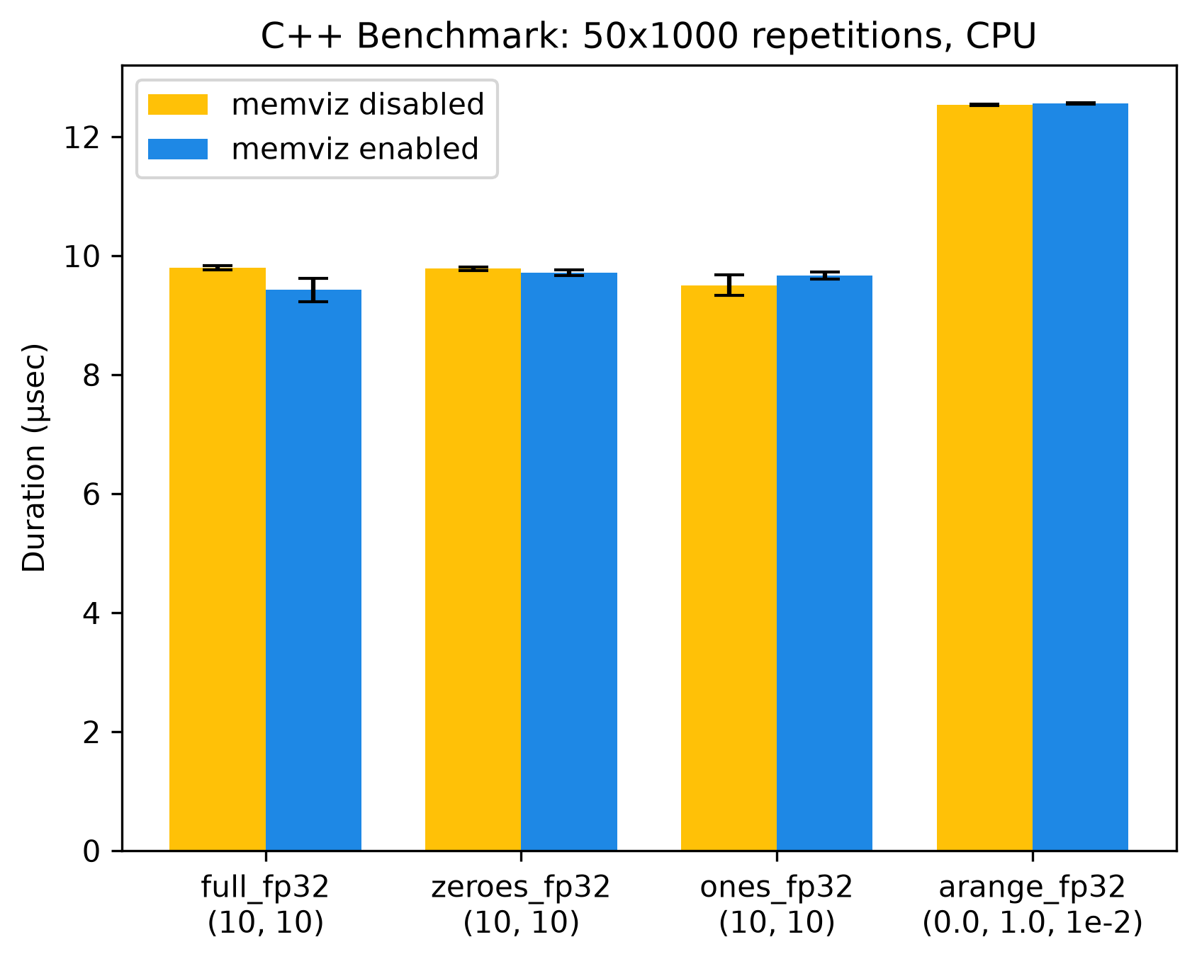
Figure 9. C++ benchmark results.
Consistent with the benchmark results we previously looked at, the difference in performance between the two conditions (recording on vs off) only seems to be impacted by noise rather than a clear event-creation overhead.